Strength and vibration analysis of transonic compressor under multiple field loads

Feng, Yu Ru; Wang, Jun Li; Li, Jin Yang

doi:10.21595/jve.2021.22151

Journal of Vibroengineering

Browse Journal

Submit article

Published: 15 May 2022

Check for updates

Strength and vibration analysis of transonic compressor under multiple field loads

Yu Ru Feng¹

Jun Li Wang²

Jin Yang Li³

^{1, 2, 3}School of Mechanical Engineering, Shaanxi University of Technology, Hanzhong, 723000, China

²Shaanxi Key Laboratory of Industrial Automation, Shaanxi University of Technology, Hanzhong, 723000, China

Corresponding Author:

Jun Li Wang

Cite the article Download PDF

Downloads 574

Abstract

The transonic axial flow compressor Rotor 37 is subjected to the combined action of thermal load, centrifugal load, and aerodynamic load in real work. The difference in load will cause the blade deformation and the size and distribution of stress to change. And it will cause the vibration frequency of the blade to change compared with the static state at room temperature. This paper studies the compressor blades based on the fluid-thermal-structure coupling method, and comprehensively considers the combined effects of thermal load, centrifugal load and aerodynamic load on the compressor blades. The results of the study show: that when the thermal load acts on the blade alone, it will have less impact on the blade deformation and greater impact on the stress, but when coupled with other loads, it will have a greater impact on the blade deformation and stress. In the case of fluid-thermal-structure coupling, the deformation of the compressor blade will first increase and then decrease with the increase of mass flow, and the change of stress will not decrease with the increase of mass flow. Rotation speed will affect the change trend of blade stress with mass flow. Compared with the static state at room temperature, the natural frequency of the blade under fluid-thermal-structure coupling has undergone a huge change. The first-order vibration frequency has increased by 25.77 %. It can be seen from the Campbell diagram that the compressor blade has a resonance at about 63 % and 98 % Point, in this case, the blade is prone to resonance, and more attention should be paid.

Strength and vibration analysis of transonic compressor under multiple field loads

Highlights

The maximum deformation of the blade occurs at the tip of the leading edge. The stress of the blade is mainly concentrated at 33% of the position of the root of the blade.
At different speeds, the deformation of the blades will first increase and then decrease with the continuous increase of the mass flow. The equivalent stress of the blades changes with the change of the mass flow and is related to the change of the speed.
In the case of fluid-thermal-structure coupling, the natural frequency of the blade has a great change compared with the natural frequency, and the first-order vibration frequency with the biggest change increases by 25.77%.
The compressor blades have a resonance point at about 63% and 98% speed.

1. Introduction

Compressor blade is one of the key parts of the engine, its safety and stability directly determine the performance of the engine. With the continuous improvement of aero-engine performance, the design trend of compressor tends to be higher pressure ratio and efficiency. However, high-speed rotating compressor blades bear large thermal stress, centrifugal force, aerodynamic force and other loads. According to the relevant data [1], compressor blade fracture accounted for more than 40 % of engine fault [2], compressor vibration fault accounted for more than 60 % of engine fault , compressor blade fault accounted for more than 70 % of vibration fault. Therefore, in order to simulate the real force of the compressor, it is necessary to comprehensively consider the influence of thermal stress, aerodynamic force and centrifugal force on the structural characteristics of the compressor, so as to obtain the force of the compressor in the real working environment.

In recent years, scholars in China and abroad have conducted a large number of studies on the compressor. In the study of the compressor flow field, Yamada and Funazaki [4] took NASA’s Rotor37 as the research object to study the interaction between the shock wave triggered by the supersonic blade and the tip leakage vortex in the tip clearance. Under the condition of standard clearance, the tip leakage vortex downstream of the shock wave breaks down under the condition of near stall. The breakdown of tip leakage vortex leads to the flow of low energy fluid downstream of shock wave in the rotor channel, resulting in a large blockage effect near the rotor tip. Zhang Yanfeng et al. [5] revealed the tip leakage characteristics of rotor Rotor 37 under near stall condition through steady and unsteady numerical simulation of Rotor 37, and further understood the influence of gap leakage flow on rotor stall.

In the aspect of fluid-structure coupling of compressor, Lee Horim et al. [6] obtained the influence of blade tip and impeller deformation on the performance of centrifugal compressor by fluid-structure coupling analysis of centrifugal compressor. Kovacevic et al. [7] used the finite element method to simulate the fluid-structure coupling of the screw compressor. The results show that the compressor will produce huge pressure difference and temperature difference on the rotor during the compression process, so that the impeller blade will be deformed. The deformation will cause the tip clearance to change, which will seriously affect the performance of the compressor. Therefore, it is necessary to carry out fluid-structure coupling simulation to study this. Tao Hailiang et al. [8] used the fluid-structure coupling method to carry out the numerical simulation of the aeroelasticity of the compressor blade, and used the unsteady fluid-structure coupling method to obtain the dynamic stress and dynamic strain analysis of the blade caused by the aerodynamic shock, so as to determine whether the compressor blade will have flutter, which provides a theoretical basis for the subsequent strength analysis. Du Zixue et al. [9] studied the influence of fluid-structure coupling field on blade strength and vibration parameters. The results show that the fluid-structure coupling has little effect on the structural strength and modal shape of the blade. Through frequency analysis, the resonant frequency of the blade is found out, which provides a basis for the optimization of the blade.

In the research of compressor temperature field, Mustafin T. N. et al. [10] designed and proposed a numerical simulation model to calculate the rotor temperature field under working condition, and analyzed the influence of structural parameters and working conditions of screw compressor on rotor temperature field. Based on fluid-thermal-structure coupling coupling, the strength analysis of a new type of gas turbine transonic compressor impeller under comprehensive load was carried out by Li Guangxin et al. [11].It is concluded that the maximum deformation of the impeller occurs at the tip of the leading edge of the splitter blade, and the maximum stress occurs at the chamfer of the back hole of the hub, which provides an engineering design calculation method for the strength analysis of the impeller and the reliable design of the compressor. Li Chunwang et al. [12] found a modal analysis method of engine blade with thermal-structure coupling prestress considering the combined effect of thermal load, centrifugal load and aerodynamic load. Wang Dingbiao et al. [13] took a centrifugal compressor impeller as the research object, and obtained the stress distribution and maximum deformation of the blade under the combined action of centrifugal force, aerodynamic force and thermal load.

When studying compressor blades, most scholars only consider the effects of centrifugal and aerodynamic loads on the blades, and less consider the thermal stress generated by gas work, so that they cannot truly reflect the deformation and stress distribution of the blade. And many scholars pay more attention to the blade shape, structure, assembly form [14] and wake-induced vibration when studying the vibration mode of the blade. However, less attention has been paid to the influence of the working environment on the natural vibration frequency and vibration shape of the blade. In actual work, factors such as centrifugal load, aerodynamic load and thermal load will change the mechanical properties of the blade material or generate prestress inside the blade, which will lead to the phenomenon of stress stiffening, and then affect the natural vibration frequency and vibration shape of the blade. In this paper, the two-way fluid-thermal-structure coupling three-field coupling method is used to simulate the compressor blades to analyze the stress and deformation of the blades under comprehensive loads, and use this as the prestress to perform modal analysis on the blades, and calculate the load And the natural frequency of the blade under no load, and finally draw the Campbell diagram of the blade to judge whether the blade will resonate. It provides reliable data for preventing blade stress damage, blade resonance, and prolonging the service life of compressor blades, and provides theoretical basis for blade structure optimization design.

2. Calculation method

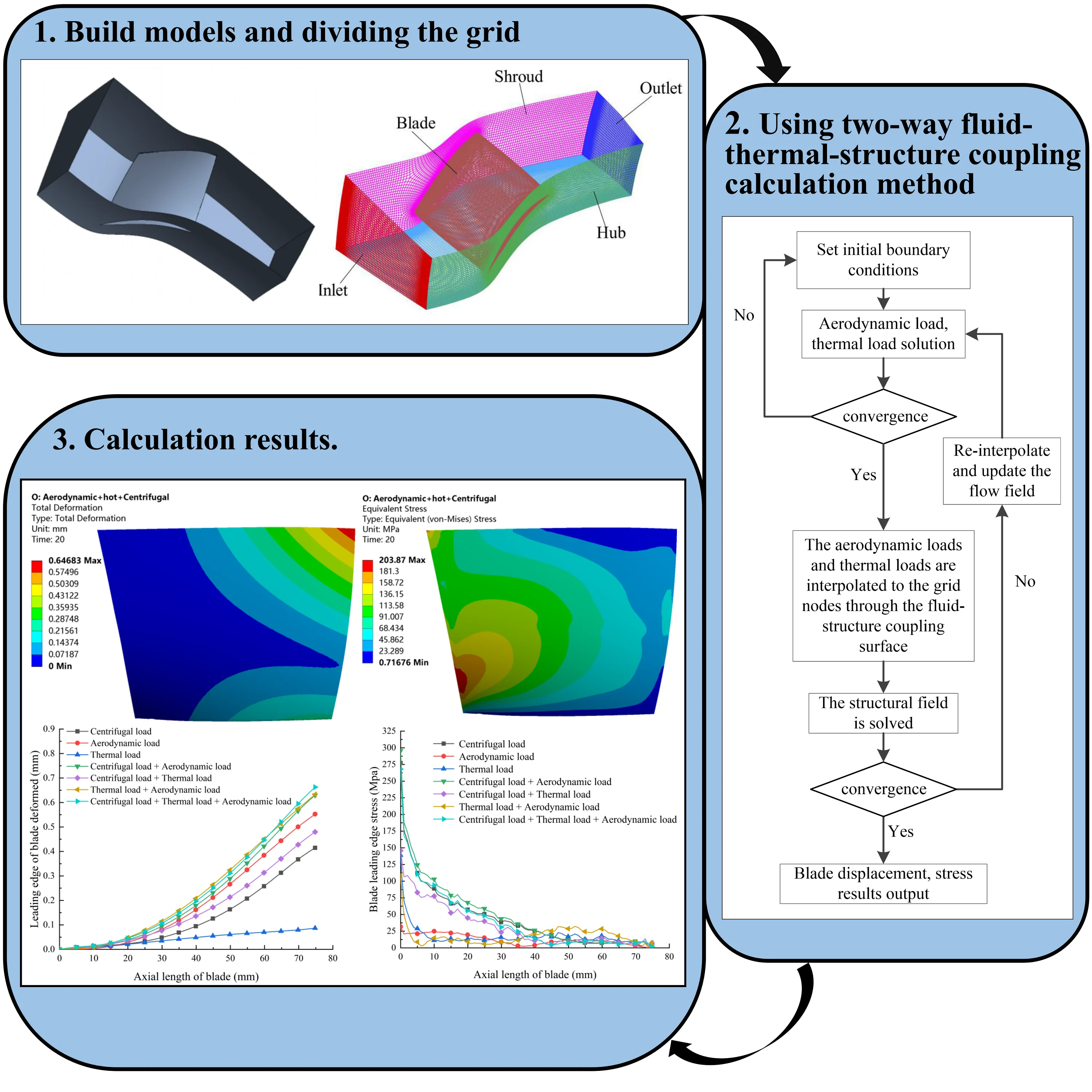
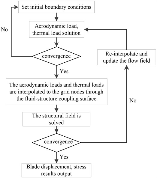
For compressor blades, the deformation of the blade caused by aerodynamic and thermal loads cannot be ignored. At the same time, the effect of blade deformation on the flow field cannot be ignored. Therefore, this paper adopts the theory of two-way fluid-thermal-structure coupling-loose coupling to numerically simulate the single-channel flow field of a transonic axial flow compressor blade. CFX solves the variables such as pressure and temperature of each grid point in the flow field, and transfers the obtained data through the coupling platform of the two on the fluid-thermal-structure coupling interface. The pressure load and thermal load are transferred from the flow field to the blade surface of the structural field. ANSYS is used to solve the structural field of each element node on the variable value, such as displacement, stress, etc. After the end of the solution, the structural displacement of the blade surface is transferred to the flow field to change the flow field distribution, and then continue to add the flow field calculation data to the structural field for calculation. In this way, when the calculation reaches local convergence, the calculation of the next time step is performed. The specific process is shown in Fig. 1.

Fig. 1Fluid-thermal-structure coupling process

3. Model establishment

3.1. Mathematical model

3.1.1. Governing equations of fluids

Fluid flow must follow the laws of conservation of physics. The basic laws of conservation include the law of conservation of mass, the law of conservation of momentum, and the law of conservation of energy [15]. If the fluid includes other mixed components, the system must also follow the law of conservation of components. For the general compressible Newtonian flow, the conservation law is described by the following governing equation.

Mass conservation equation:

1

\frac{\partial ρ_{f}}{\partial t} = \nabla \cdot (ρ_{f} v) = 0 .

Momentum conservation equation:

2

\frac{\partial ρ_{f}}{\partial t} = \nabla \cdot (ρ_{f} v v - τ_{f}) = f_{f} .

Among them, $t$ represents time and $f_{f}$ is the volumetric force vector. $p_{f}$ is the fluid density, $v$ is the fluid velocity vector, and $τ_{f}$ is the shear force tensor, which can be expressed as Eq. (3):

3

τ_{f} = (- p + u \nabla \cdot v) I + 2 u e,

where, $p$ is fluid pressure, $u$ is dynamic viscosity, $e$ is velocity stress tensor:

4

e = \frac{1}{2} (\nabla v + \nabla v^{T}) .

3.1.2. Governing equations of structures

For the solid field is mainly the deformation of the solid caused by the action of the fluid force in the fluid field, the conservation equation of the solid part can be derived from Newton’s second law:

5

ρ_{s} {\ddot{d}}_{s} = \nabla \cdot σ_{s} + f_{s},

where $p_{s}$ is the density of structures, $σ_{s}$ is the Cauchy stress tensor, and $f_{s}$ is the volume force vector. ${\ddot{d}}_{s}$ is the local acceleration vector in the structure domain:

6

\frac{\partial (ρ h_{t o t})}{\partial t} - \frac{\partial p}{\partial t} + \nabla \cdot (ρ_{f} v h_{t o t}) = \nabla \cdot (λ \nabla T) + \nabla \cdot (v \cdot τ) + v \cdot ρ f_{f} + S_{E},

where, $λ$ represents the thermal conductivity, and $S_{E}$ represents the energy source term.

For the structure part, the thermal deformation term caused by temperature difference is added. Its mathematical expression is as shown in Eq. (7):

7

f_{T} = α_{T} \cdot \nabla T,

where $α_{T}$ is the thermal expansion coefficient dependent on temperature.

3.1.3. Fluid-structure interaction coupling equation

Fluid-structure coupling follows the most basic principle of conservation, so it is at the interface of fluid-structure coupling. Should satisfy the fluid and solid stress ( $τ$ ), displacement ( $d$ ), heat flow ( $q$ ), temperature ( $T$ ) and other variables are equal [16], that is, Eq. (8) is satisfied:

8

\{\begin{array}{l} τ_{f} \cdot n_{f} = τ_{s} \cdot n_{s}, \\ d_{f} = d_{s}, \\ q_{f} = q_{s}, \\ T_{f} = T_{s} . \end{array}

In Eq. (8), subscript $f$ stands for fluid, and the subscript $s$ stands for solid.

3.1.4. Thermal-structure coupling equation

The temperature field and thermoelastic finite element equation of the thermosetting unidirectional calculation model are as follows:

9

M \frac{\partial T}{\partial t} + K T - Q = 0,

10

D U = G T + F .

In Eq. (9) and Eq. (10), $M$ is the heat capacity matrix; $T$ is the temperature vector; $t$ is the time; $K$ is the heat conduction matrix; $Q$ is the heat flow vector; $D$ is the stiffness matrix; $U$ is the displacement vector; $G$ is the thermal stress coefficient matrix; $F$ is the mechanical force vector.

3.1.5. Basic theory of compressor blade modal analysis

Modal analysis is a technique used to determine the vibration characteristics of a structure. The main application is to establish a predictive model of the dynamic response of the structure to serve the dynamic strength design of the structure. For a multi-degree-of-freedom vibration system, the dynamics of the elastic structure can be solved according to the D'Alembert principle to derive the dynamic balance equation [17]:

11

[M] \{\ddot{u}\} + [C] \{\dot{u}\} + [K] \{u\} = \{F (t)\},

where: $[M]$ is the mass matrix; $[C]$ is the damping matrix; $[K]$ is the stiffness matrix; $\{\ddot{u}\}$ is the acceleration vector; $\{\dot{u}\}$ is the velocity vector, $u$ is the displacement vector; $F (t)$ is the force vector.

3.2. Physical model

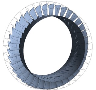
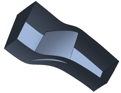
The research object of this paper is the NASA rotor Rotor37, which was originally designed and tested by Reid and Moore of Glenn Research Center in the United States. The design parameters and experimental data can be found in reference [19]. Rotor37 is the rotor in Stage37 of a four-stage axial compressor with a high boost ratio (20:1). The geometric parameters are shown in Table 1. Fig. 2 is a schematic diagram of the single-channel model of the rotor.

Table 1Basic design geometrical parameters of rotor

Parameter	Design value
Total rotor pressure ratio	2.106
Total rotor temperature ratio	1.261
The adiabatic efficiency	0.877
Apical clearance / mm	0.356
Design mass flow / (kg∙s^-1)	20.188
Design speed / (r∙min^-1)	17188.7
Leaf number	36

The research object of this paper is the NASA rotor Rotor 37, which was originally designed and tested by Reid and Moore from Glenn Research Center in the United States. The design parameters and experimental data can be found in the reference. Rotor 37 is a rotor in a four-stage axial compressor Stage 37 with a high pressurization ratio of 20:1. The geometrical parameters are shown in Table 1. Fig. 2 is a schematic diagram of the rotor mode, Fig. 2(a) is a full-channel model, Fig. 2(b) is a single-channel model.

Fig. 2Sketch of Rotor 37 model

a) Pressure ratio characteristic curve

b) Efficiency characteristic curve

3.3. Meshing and independence verification

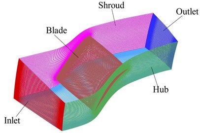
This paper uses the TurboGrid software in ANSYS Workbench to divide the grid. When dividing the grid, all the inlet and outlet sections of the calculation domain are extended to the outer diameter of the casing to prevent the reflected pressure wave at the inlet and outlet boundaries from generating the internal flow of the compressor. Influence. In this paper, the rotor blade channel adopts H-O-H structured grid, the blade adopts O-shaped grid, the inlet and outlet adopt H-shaped grid, and the gap adopts a combined butterfly-shaped and H-shaped grid structure. Increase the number of meshes near the wall and the tip of the blade to refine the mesh.

The number of grids directly affects the accuracy of the numerical simulation. Too many grids will increase the amount of calculation, and too few grids will cause the calculation results to be distorted. In order to verify whether the grid density is reasonable, five sets of grids are drawn separately. In order to save computing resources, according to the research results of the literature [18], grids with 258000, 456000, 741200, 1.068 million, and 1.56 million nodes were selected to verify the grid independence of the flow field. It can be seen from Fig. 3 that as the number of grids increases, the isentropic efficiency gradually increases, but when the number of grids reaches a certain value, the isentropic efficiency does not change with the increase of the number of grids. It can be seen from Fig. 3 that when the number of nodes is greater than 741200, the isentropic efficiency does not show a significant change. Table 2 shows the comparison between the isentropic efficiency obtained by numerical simulation and the experimental value under different grid numbers. It can be seen from Table 2 that when the number of nodes is greater than 741200, the isentropic efficiency does not change significantly with the increase of the grid, and the error of isentropic efficiency with the experimental design point is 2.3 %. Therefore, it can be considered that the number of nodes has reached the requirement of grid independence. For reasonable calculation accuracy and calculation speed, this paper selects a grid with a total number of 741200 for the numerical calculation of the blade flow field. Fig. 4 shows the runner grid.

Table 2Comparison of numerical simulation results with experimental values

Grid number	Experiment / %	Simulation / %	Error / %
25.8w	87.7	84.35	3.82
45.6w	87.7	84.65	3.47
74.12w	87.7	85.68	2.30
106.8w	87.7	85.61	2.38
150w	87.7	85.72	2.25

Fig. 3Grid independence verification

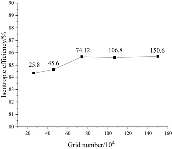
Fig. 4Port grid

3.4. Moving mesh model

In the process of fluid-thermal-structure coupling solution, the deformation of the structure motion will change the flow field. Therefore, in the process of numerical simulation, the CFD grid must change with the deformation of the structure. In the iterative process of calculation at each time step, the finite volume grid in the CFD calculation domain must follow the structure to adapt to a new position and be solved in a new state. The dynamic grid is the entire process of solving at each time step, the blade vibration displacement causes the shape of the flow field to change, and the CFD grid must follow the structure to adapt to the new position. In this paper, we use CFX software to realize the movement of the grid, that is, the dynamic grid. In the calculation process, the grid node displacement changes on the coupled interface are obtained by interpolation of the blade surface vibration displacement. At the same time, in order to avoid serious grid deformation, the grid quality will be reduced and the calculation static will be affected. The flow field grid nodes around the blade are also Displacement must be generated accordingly. Before each flow field is iteratively calculated, the node displacement change is obtained by solving the mesh displacement equation, and then the coordinate value of the mesh node is updated to form a new flow field grid.

3.5. Solve settings

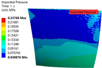
In the process of numerical simulation, given the back pressure at the design point, the back pressure is gradually reduced. When the outlet flow does not change, this point is regarded as the blocking point of the rotor. On the contrary, gradually increase the back pressure and regard the last convergence point as the near stall point of the rotor. The turbulence model of the axial compressor blade calculation is K-W-SST [21], the inlet boundary conditions: total temperature 288.15K, total pressure 101325 Pa, outlet given back pressure, the simplified radial balance is used to obtain the back pressure along the span direction Distribution. The solid wall adopts no-slip boundary condition. The compressor blades are made of TC4 (Ti-6Al-4V) material, and the pressure field and temperature field obtained by the flow field calculation are loaded on the blades. Figs. 5, 6 show the compressor temperature field and pressure field loading conditions when the compressor outlet back pressure is 0.12 MPa at rated speed. The maximum pressure reaches 0.23768 MPa and the maximum temperature reaches 112.11 ℃.

Fig. 5Pressure field loading of compressor blade

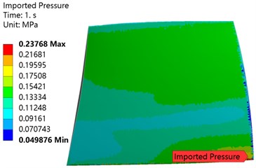
a) Pressure surface

b) Suction surface

Fig. 6Temperature field loading of compressor blades

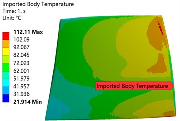
a) Pressure surface

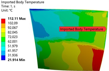
b) Suction surface

3.6. Model validation

Combining experiments and classic literature to verify the accuracy of the results, Fig. 7 shows the compressor characteristic curve. After calculation, the design point pressure ratio of the numerical calculation has an error of 3.84 % compared with the experimental value [20].

Fig. 7Comparison of calculated results and experimental results

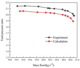
a) Pressure ratio characteristic curve

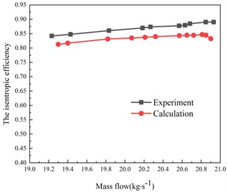
b) Efficiency characteristic curve

The value of the isentropic efficiency is compared with the experimental value. The error is 2.3 %. However, the variation trend of numerical calculation and experimental results is basically the same, and the error is also within the acceptable range. The error may be related to the selected turbulence model and insufficient accuracy of the Rotor37 data. According to the experimental data in literature [19], at the design speed, the clogging flow of the rotor is 20.93 kg/s, and the calculated value in this paper is 20.9 kg/s, the difference between the two is 0.14 %. In addition, the stall of the rotor the flow rate is 19.36 kg/s, the calculated value predicted in this article is 19.3 kg/s, the difference between the two is 0.30 %. It can be seen that the calculation method in this paper can predict the stall boundary and blockage boundary of the rotor more accurately.

4. Result analysis

In order to understand the effect of different loads on the deformation and stress of the blade more clearly, this paper analyzes based on the following situations, 1) only consider the blade’s aerodynamic load on the flow field, 2) only consider the blade’s centrifugal load, 3) only consider the blade heat Load effect; 4) consider the coupling effect of different loads.

First analyze the deformation and stress of the blade under a single load. From Table 3, we can see that the deformation when the blade is only subjected to thermal load is very small compared to the other two cases, but the largest equivalent effect is produced. The force is relatively large, and the equivalent stress caused by aerodynamic load is relatively small. That is, aerodynamic load and centrifugal load are the main factors affecting blade deformation, and thermal load and centrifugal load are the main factors affecting blade stress. Therefore, we cannot ignore the influence of thermal load on blade deformation and stress when we calculate.

Table 3Maximum deformation and maximum stress of blade under single load

The load	The biggest deformation (mm)	Maximum equivalent stress (MPa)
Only subjected to aerodynamic load	0.58938	57.16
Only under thermal load	0.060304	258.67
Centrifugal loads only	0.41516	277.41

4.1. Blade deformation distribution under different loads

In order to understand the deformation distribution of the blade under different loads, this paper couples different loads to analyze the deformation and stress of the blade. It can be seen from the blade deformation cloud diagram of the blade under different load conditions in Fig. 8 that no matter what kind of load the blade is subjected to, the deformation of the blade gradually increases with the increase of the blade height, and the maximum deformation occurs at the tip of the leading edge. Referring to Table 3, it can be seen that after the thermal load is added, the deformation distribution and size of the blade have changed to different degrees in comparison with only a single load. After the centrifugal load is added to the thermal load, the maximum deformation of the blade increases by 15.63 %. After the aerodynamic load is added to the thermal load, the maximum deformation of the blade increases by 14.56 %. The combined load deformation caused by aerodynamic and centrifugal load has increased by 2.68 % compared with the previous maximum deformation after thermal load is added. Comparing Table 3, it can be found that when the blade is only subjected to thermal load, the deformation produced is very small, but when the thermal load is coupled with other loads and then applied to the blade, the blade deformation has a different degree than that of a single load. However, the influence of thermal load on the deformation of compressor blades is less than that of aerodynamic load and centrifugal load.

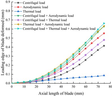
In order to understand the deformation distribution of the blade more clearly, a path is set up on the leading edge of the blade to track the deformation distribution of the leading edge of the blade from the root to the tip. It can be seen from Fig. 9 that no matter what load the blade bears, the deformation of the blade gradually increases from the root to the tip, and reaches the maximum at the leading edge of the tip. The deformation of the blade is close to zero due to only the thermal load. It can be seen from the Fig. 9 that when the blade is subjected to aerodynamic load or coupled with other loads, the deformation of the blade is relatively large, that is, the aerodynamic load is the main factor that affects the deformation of the blade. The maximum deformation of the blade caused by the combined action of the thermal load, centrifugal load and aerodynamic load of the blade is the largest, and it appears at the tip of the leading edge of the blade, which also corresponds to the blade deformation cloud diagram in Fig. 8. When the thermal load is coupled with other loads, the deformation of the blade will increase to different degrees. Therefore, when studying the deformation of the blade, the influence of the thermal load on the blade deformation cannot be ignored.

Fig. 8Deformation cloud diagram of blade under different load coupling

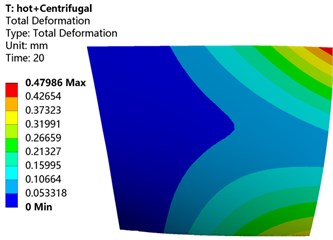
a) Centrifugal load + thermal load

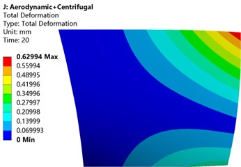
b) Centrifugal load + aerodynamic load

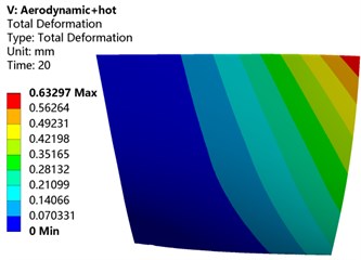
c) Aerodynamic load + thermal load

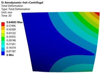
d) Aerodynamic load + centrifugal load + thermal load

Fig. 9Variations of blade deformation along the path of the leading edge under coupling of different loads

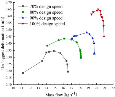
From the above research, it can be seen that the deformation of the blade based on the fluid-thermal-structure coupling is most in line with the actual load condition of the blade. This paper also studies the change of blade deformation with mass flow under different design speeds, that is, the blade runs from near-blocking condition to near-stall condition. It can be seen from Fig. 10 that under the combined action of thermal load, centrifugal load, and aerodynamic load, the maximum deformation of the blade at 100 % design speed shows a trend of first increasing and then gradually decreasing with the increase of mass flow. When the flow is 20.32 kg·s-1, the maximum deformation of the blade reaches its peak value, which is 0.65047 mm. From this point on, the maximum deformation of the blade gradually decreases as the mass flow increases. It can be seen from the Fig. 10 that the maximum deformation of the blade with mass flow at other design speeds is basically the same as the 100 % design speed. The maximum deformation of the blade shows a trend of first increasing and then decreasing with the continuous increase of mass flow. There will be a peak at a certain flow. The maximum deformation of the blade increases with the increase of the speed, and the maximum deformation near the stall point is greater than the near jam point at the same speed.

Fig. 10Variation of blade deformation with mass flow at different speeds

4.2. Blade stress distribution under different loads

Fig. 11 shows the stress distribution of the blade under different load conditions. The area with larger stress is mainly concentrated in the 33 % position of the root of the blade, and then spreads radially to the surrounding and gradually decreases. Comparing Table 3, it can be seen that after the thermal load is added, the comparison is only affected by a single load, and the stress distribution and size of the blade have changed to different degrees. After the centrifugal load is added to the thermal load, the maximum equivalent stress of the blade is reduced by 28.45 %. After the aerodynamic load is added to the thermal load, the maximum equivalent stress of the blade is increased by nearly 2.97 times. The maximum equivalent stress generated by the aerodynamic and centrifugal load after the thermal load is reduced by 31.07 % compared to the aerodynamic and centrifugal load alone. This shows that the thermal load has an impact on the stress distribution and size of the blade, and the impact is greater.

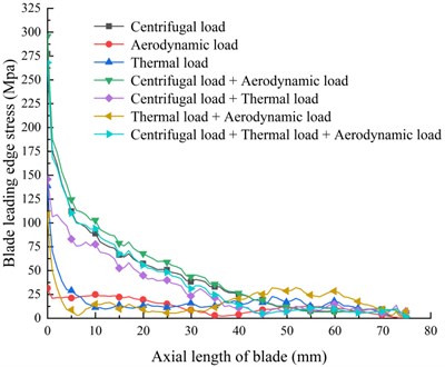
Fig. 12 shows the stress distribution at the leading edge of the blade under different load conditions. It can be seen from the figure that the stress at the leading edge of the blade is the largest under the combined action of centrifugal load and aerodynamic load, reaching 295.77 MPa. At the leading edge of the blade, the stress at the root of the blade reaches the maximum, and it gradually decreases from the root to the tip, and the amount of reduction gradually decreases. When it is close to the tip, the stress is small and almost zero. This is the same as the blade stress trend in Fig. 11.

Fig. 11Equivalent stress cloud diagram of blade under different load coupling

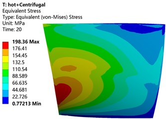
a) Centrifugal load + thermal load

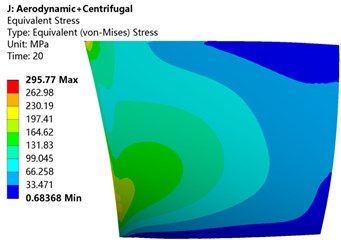
b) Centrifugal load + aerodynamic load

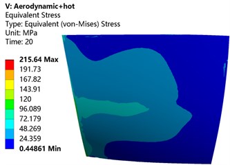
c) Aerodynamic load + thermal load

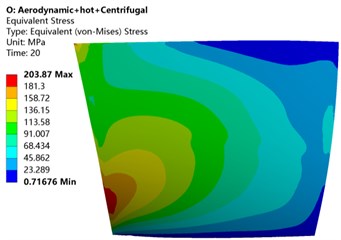
d) Aerodynamic load + centrifugal load + thermal load

Fig. 12Variation of blade equivalent stress along the path of the leading edge under different load coupling

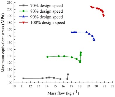
It can be seen from Fig. 13 that the stress of the blade at 100 % design speed and 90 % design speed changes regularly with the change of mass flow. It can be seen from the figure that the maximum equivalent stress of the blade appears at 100 % design speed. At the near stall point, it reached 203.968 MPa. The equivalent stress of the blade shows a decreasing trend with the continuous increase of the mass flow, and with the gradual increase of the mass flow, that is, when the operating conditions of the blades move closer to the clogging conditions, the amount of decrease gradually increases. But when the speed drops to 80 % of the design speed and 70 % of the design speed, the change trend of the maximum equivalent stress of the blade changes, instead of a single decrease with the increase of the flow rate. From the beginning, it changes slowly with the increase of mass flow, and when it runs to the operating condition near the blocking point, the maximum equivalent stress of the blade begins to increase gradually. The maximum equivalent stress of the blades increases continuously with the increase of the speed. It can be seen that the change trend of the maximum equivalent stress of the blade with the mass flow will change with the change of the speed. We should pay more attention when studying the strength of the blade.

It can be seen from the above analysis that when we analyze and check the strength of the blade, we must take the thermal load into account. That is, we must consider the combined effect of thermal load, centrifugal load and aerodynamic load to be able to simulate the working conditions of the blade to the greatest extent.

Fig. 13Variation of blade equivalent stress with mass flow at different speeds

4.3. Modal analysis and resonance judgment of blades under different prestresses

The modal analysis of the blade under actual working conditions is to use the comprehensive stress generated by the aerodynamic load, thermal load and centrifugal load on the blade in actual work as the prestress to perform the modal analysis on the blade. After considering the effect of aerodynamic load on the blade, the natural frequencies of the first and third orders of the blade increase, and the natural frequencies of the second, fourth, fifth, and sixth orders are reduced to varying degrees. That is, after the introduction of aerodynamic force, the frequency of the main mode of bending of the blade increases, and the frequency of the main mode of torsion decreases. It can be seen from Table 4 that when considering the effect of aerodynamic load or thermal load on the blade, the natural frequency of each order of the blade has changed compared to the natural frequency without considering any load, but the amplitude of the change is very small, and the maximum change does not exceed 0.5 %, which is compatible with the natural frequency generated by the combined load of the blade subjected to the thermal load and the aerodynamic load. It can be seen from this that the aerodynamic load and the thermal load are not the main factors affecting the natural frequency of the blade. In contrast, when only considering the effect of centrifugal load on the blade, the natural frequency of the blade has a significant increase compared to the natural frequency under no load, and the first-order frequency is increased by 25.77 %. It can be seen from the table that as long as there is a centrifugal load in the load on the blade, the natural frequency of the blade has a significant increase. It can be seen that the centrifugal load is the main factor affecting the natural frequency of the blade, and the aerodynamic load and thermal load are secondary factor.

For rotating machinery, if the natural frequency of the blade is the same as or close to the excitation frequency generated by the system during rotation, it will cause the blade to resonate, produce larger amplitude and vibration stress, and easily cause high-cycle or low-cycle fatigue fracture. Campbell diagram can determine whether the frequency of the various excitation forces generated by the rotating parts of the compressor within the operating speed range of the compressor is consistent with the natural frequency of some parts [22], [23], which can effectively prevent the occurrence of resonance and damage to the parts. Based on the thermal load, aerodynamic load and centrifugal load prestress, the modal analysis of the blades at different speeds is carried out, and the natural frequencies of the blades at different speeds are obtained as shown in the Table 5. Through the natural frequency at different speeds, different speed lines, and the compressor’s excitation force data [17], a Campbell diagram can be drawn, as shown in Fig. 14.

Table 4Design the natural frequency of the blade under different loads

Natural frequencies under different loads (Hz)	Modal order number
Natural frequencies under different loads (Hz)	1 order	2 order	3 order	4 order	5 order	6 order
No load	926.5	2608	3324.3	4975.6	6197.5	6896.3
Aerodynamic	929.01	2600	3327.1	4966.3	6161.7	6894.6
Centrifugal	1165.3	2651.1	3571.2	5027.8	6277.4	7109.2
Thermal	926.66	2608	3324.7	4973.2	6194.7	6890.5
Centrifugal + Pneumatic	1166.2	2649.1	3573.3	5028.3	6278.3	7112.5
Centrifugal + thermal	1165.2	2649.1	3570.3	5026.3	6276	7103.2
Thermal + pneumatic	929.16	2597.7	3326.2	4964.5	6189.3	6888.9
Centrifugal + pneumatic + thermal	1166.1	2648	3571.2	5024.6	6275.4	7103.2

Table 5The first 6 natural frequencies of blades at different speeds

Order time	Frequency (Hz)
Order time	70 % design speed	80 % design speed	90 % design speed	100 % design speed
1	1051.7	1086.7	1125	1166.1
2	2626.3	2632.8	2641	2648
3	3449.3	3486.1	3527.3	3571.2
4	5000	5007.9	5017.9	5024.6
5	6237.3	6248.8	6261.9	6275.4
6	7001.3	7032.2	7068.8	7103.2

From the Campbell diagram of the blade, we can see that not all speeds will become the dangerous speed conditions of the blade. From the figure, it can be seen that there is a resonance point of the blade at 63 % speed and 98 % speed. Resonance is prone to occur at 100 % speed, causing damage to the blades.

Fig. 14Compressor blade Camber diagram

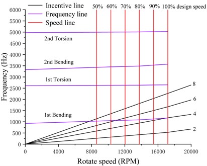
As can be seen from the Campbell diagram of the blade, not all rotating speeds will become dangerous rotating speed conditions of the blade. As can be seen from the figure, there is a resonance point around 63 % rotating speed and 98 % rotating speed of the blade, which indicates that the blade is prone to resonance at 100 % rotating speed, leading to damage to the blade. The solution to blade resonance is to change the structure of the blade so as to change the natural frequency of the blade or change the speed of the compressor, so as to avoid the vibration speed close to the natural frequency. The method to solve the blade resonance: change the structure of the blade to change the natural frequency of the blade or change the speed of the compressor, so as to avoid the resonance point speed close to the natural frequency.

5. Conclusions

Based on the CFD/CSD fluid-thermal-structure coupling method, this paper analyzes the influence of the aerodynamic load, thermal load and centrifugal load of the transonic axial flow compressor on the structural characteristics of the blade. The deformation and stress of the compressor blade in the case of solid coupling, and the influence of different loads on the structural characteristics of the compressor blade are analyzed. The blade is modal analysis under prestress, and the Campbell diagram of the blade is obtained. The main conclusions are obtained. as follows:

1) The maximum deformation of the blade occurs at the tip of the leading edge, and only the thermal load has less influence on the blade deformation than aerodynamic load and centrifugal load. However, when the thermal load is coupled with other loads, it will have a greater impact on the deformation of the compressor blades. The stress of the blade is mainly concentrated at 33 % of the position of the root of the blade, and the thermal load has an impact on the stress distribution and size of the blade, and the influence is relatively large. The influence of thermal load on the structural characteristics of the compressor blades cannot be ignored.

2) At different speeds, the deformation of the blades will first increase and then decrease with the continuous increase of the mass flow. The equivalent stress of the blades changes with the change of the mass flow and is related to the change of the speed. We are designing and Pay more attention when inspecting.

3) Considering the actual working conditions of the compressor, the natural frequency of the blade obtained by thermal load, centrifugal load and aerodynamic load has a huge change compared with no load. The first-order vibration frequency with the largest change increases by 25.77 %. Therefore, in the modal analysis of the blade, it is necessary to comprehensively consider the impact of various loads on the blade, and conduct a modal analysis based on fluid-thermal-structure coupling prestress.

4) The compressor blades have a resonance point at about 63 % and 98 % speed. In this case, the blades are prone to resonance, and more attention should be paid in the later analysis.

References

G. Cheng, Analysis of Aeroengine Structural Design. (in Chinese), Beijing, China: Beijing University of Aeronautics and Astronautics Press, 2014.

Search CrossRef
L. Zhang et al., “Vibration analysis of the compressor blade in a gas turbine,” (in Chinese), Journal of Engineering for Thermal Energy and Power, Vol. 34, No. 1, pp. 34–39, 2019, https://doi.org/10.16146/j.cnki.rndlgc.2019.01.006

Publisher
X. M. Jin et al., “Analysis of integrated centrifugal impeller blade vibration reliability,” (in Chinese), Journal of Aerospace Power, Vol. 19, No. 5, pp. 610–613, 2004, https://doi.org/10.3969/j.issn.1000-8055.2004.05.006

Publisher
K. Yamada, K. Funazaki, and M. Furukawa, “The behavior of tip clearance flow at near-stall condition in a transonic axial compressor rotor,” in ASME Turbo Expo 2007: Power for Land, Sea, and Air, Jan. 2007, https://doi.org/10.1115/gt2007-27725

Publisher
Y. F. Zhang, W. L. Chu, and X. G. Lu, “Numerical simulation of the flow characteristic of tip leakage flow in a transonic axial-flow compressor at near stall condition,” (in Chinese), Journal of Aerospace Power, Vol. 23, No. 7, pp. 1293–1298, 2008.

Search CrossRef
H. Lee, C. Kim, J. Yang, C. Son, Y. Hwang, and J. Jeong, “Study on the performance of a centrifugal compressor using fluid-structure interaction method,” (in Korean), Transactions of the Korean Society of Mechanical Engineers B, Vol. 40, No. 6, pp. 357–363, Jun. 2016, https://doi.org/10.3795/ksme-b.2016.40.6.357

Publisher
A. Kovacevic, N. Stosic, and I. K. Smith, “Numerical simulation of fluid flow and solid structure in screw compressors,” in ASME 2002 International Mechanical Engineering Congress and Exposition, Jan. 2002, https://doi.org/10.1115/imece2002-33367

Publisher
H. L. Tao et al., “Numerical simulation of aeroelastic response in compressor based on fluid-structure interaction coupling,” (in Chinese), Journal of Aerospace Power, Vol. 27, No. 5, pp. 1054–1060, 2012.

Search CrossRef
Z. X. Du et al., “Fluid-structure interaction strength and vibration of compressor blade,” (in Chinese), Measurement and Diagnosis, Vol. 33, No. 5, pp. 789–793, 2013, https://doi.org/10.3969/j.issn.1004-6801.2013.05.010

Publisher
T. N. Mustafin, R. R. Yakupova, A. V. Burmistrova, M. S. Khamidullina, and I. G. Khisameeva, “Analysis of influence of screw compressor construction parameters and working condition on rotor temperature fields,” Procedia Engineering, Vol. 152, pp. 423–433, 2016, https://doi.org/10.1016/j.proeng.2016.07.612

Publisher
G. X. Li, Z. D. Zhang, and X. P. Shu, “Strength analysis of gas turbine compressor impeller based on fluid-thermal-structure interaction,” (in Chinese), Fluid Machinery, Vol. 45, No. 4, pp. 36–40, 2017.

Search CrossRef
C. W. Li et al., “Modal analysis of aero-engine blade based on thermal-structure coupling pre-stressing force,” (in Chinese), Journal of Air Force Engineering University: Natural Science Edition, Vol. 17, No. 2, pp. 1–4, 2016, https://doi.org/10.3969/j.issn.1009-3516.2016.02.001

Publisher
D. B. Wang et al., “Simulation research on impeller blade of centrifugal compressor based on fluid-structure interaction coupling,” (in Chinese), Journal of Thermal Science and Technology, Vol. 19, No. 1, 2020, https://doi.org/10.13738/j.issn.1671-8097.018218

Publisher
Y. H. Xi et al., “Experimental study on vibration characteristics of a steam tutbine blade with in Tegnal Shroud and Tie Wirez,” (in Chinese), Turbine Technology, Vol. 53, No. 5, pp. 81–84, 2011, https://doi.org/10.3969/j.issn.1001-5884.2011.02.001

Publisher
F. J. Wang, Computational Fluid Dynamics Analysis. (in Chinese), Beijing, China: Tsinghua University Press, 2004, pp. 7–9.

Search CrossRef
X. G. Song, L. Cai, and H. Zhang, Ansys fluid-structure interaction Coupling Analysis and Engineering Examples. (in Chinese), Beijing, China: China Water Conservancy and Hydropower Press, 2012, pp. 3–5.

Search CrossRef
M. F. Zhang, “Static and modal analysis of compressor blade based on fluid-structure interaction interaction,” (in Chinese), Harbin Engineering University, 2016.

Search CrossRef
X. G. Lu, “Study on internal flow instability and passive control strategy of axial flow compressor,” (in Chinese), Northwestern Polytechnical University, 2007.

Search CrossRef
L. Reid and R. D. Moore, “Design and overall performance of four highly loaded, high speed inlet stages for an advanced high-pressure-ratio core compressor,” NASA TP-1337, Sep. 2013, http://ntrs.nasa.gov/search.jsp?r=19780025165

Search CrossRef
S.-I. Nam, R. Stein, H. Grobe, and H. Hubberten, “Late Quaternary glacial-interglacial changes in sediment composition at the East Greenland continental margin and their paleoceanographic implications,” Marine Geology, Vol. 122, No. 3, pp. 243–262, Jan. 1995, https://doi.org/10.1016/0025-3227(94)00070-2

Publisher
J. Pi et al., “Stall and surge simulation of 3D axial compressor rotor based on Ansys CFX,” (in Chinese), Journal of Machine Design, Vol. 32, No. 1, 2015, https://doi.org/10.13841/j.cnki.jxsj.2015.01.021

Publisher
J. H. Zhang et al., “Numerical study on vibration characteristics of axial flow compressor blades under fluid-structure interaction interaction,” (in Chinese), Journal of Vibration, Vol. 38, No. 1, 2018, https://doi.org/10.16450/j.cnki.issn.1004-6801.2018.01.009

Publisher
Y. Liu, C. Yang, C. Ma, and D. Lao, “Forced responses on a radial turbine with nozzle guide vanes,” Journal of Thermal Science, Vol. 23, No. 2, pp. 138–144, Apr. 2014, https://doi.org/10.1007/s11630-014-0688-4

Publisher

About this article

Received

12 July 2021

Accepted

27 November 2021

Published

15 May 2022

SUBJECTS

Flow induced structural vibrations

DOI

https://doi.org/10.21595/jve.2021.22151

Keywords

transonic axial compressor

fluid-thermal-structure coupling

stress

strain

Acknowledgements

This work was supported by the Science Technology Department Key Project of Shaanxi Province (No. 2017ZDXM-GY-138), Key Project of Shaanxi Provincial Department of Science and Technology (No. 2019TSLGY02-03), General Project of Shaanxi Provincial Department of Science and Technology (No. 2020JM-600), and Shaanxi Provincial Department of Education Scientific Research Project (19JK0172).

This is an open access article distributed under the Creative Commons Attribution License, which permits unrestricted use, distribution, and reproduction in any medium, provided the original work is properly cited.

Previous article in issue Previous Next article in issue Next

Research article

2022 08 25

Influence of tip leakage flow on the aerodynamic damping of compressor blade torsional vibration

Xiang Zhang, Xiao Guo, Guozhe Ren

Research article

2022 01 30

Vibration characteristics of axial compressor blade under complex loads

Xi Fu, Yun Liu, Junhong Zhang, Wenzhao Yang

Research article

2021 11 11

Characteristics of embedded triple screw pump based on thermal-fluid-structure coupling

Bowen Zhu, Yongqiang Zhao, Hongling Hou, Zhehui Li

Research article

2021 04 01

Structural optimization of H-type VAWT blade under fluid-structure interaction conditions

Xu Zhang, Zituo Wang, Wei Li

Y. R. Feng, J. L. Wang, and J. Y. Li, “Strength and vibration analysis of transonic compressor under multiple field loads,” Journal of Vibroengineering, Vol. 24, No. 3, pp. 550–566, May 2022, https://doi.org/10.21595/jve.2021.22151

Copy Extrica

Copied to clipboard!

TY  - JOUR
DO  - 10.21595/jve.2021.22151
UR  - https://doi.org/10.21595/jve.2021.22151
TI  - Strength and vibration analysis of transonic compressor under multiple field loads
T2  - Journal of Vibroengineering
AU  - Feng, Yu Ru
AU  - Wang, Jun Li
AU  - Li, Jin Yang
PY  - 2022
DA  - 2022/01/25
PB  - JVE International Ltd.
SP  - 550-566
SN  - 1392-8716
SN  - 2538-8460
ER  - 

Copy Ris

Copied to clipboard!

@article{Feng_2022,
	doi = {10.21595/jve.2021.22151},
	url = {https://doi.org/10.21595/jve.2021.22151},
	year = 2022,
	month = {jan},
	publisher = {{JVE} International Ltd.},
	pages = {550--566},
	author = {Yu Ru Feng and Jun Li Wang and Jin Yang Li},
	title = {Strength and vibration analysis of transonic compressor under multiple field loads},
	journal = {Journal of Vibroengineering}
}

Copy Bibtex

Copied to clipboard!

[1]Y. R. Feng, J. L. Wang, and J. Y. Li, “Strength and vibration analysis of transonic compressor under multiple field loads,” Journal of Vibroengineering, pp. 550–566, Jan. 2022, doi: 10.21595/jve.2021.22151.

Copy IEEE

Copied to clipboard!

Feng, Yu Ru, Jun Li Wang, and Jin Yang Li. “Strength and Vibration Analysis of Transonic Compressor under Multiple Field Loads.” Journal of Vibroengineering, January 25, 2022, 550–66. https://doi.org/10.21595/jve.2021.22151.

Copy Chicago

Copied to clipboard!

Strength and vibration analysis of transonic compressor under multiple field loads

Abstract

Highlights

1. Introduction

2. Calculation method

3. Model establishment

3.1. Mathematical model

3.1.1. Governing equations of fluids

3.1.2. Governing equations of structures

3.1.3. Fluid-structure interaction coupling equation

3.1.4. Thermal-structure coupling equation

3.1.5. Basic theory of compressor blade modal analysis

3.2. Physical model

3.3. Meshing and independence verification

3.4. Moving mesh model

3.5. Solve settings

3.6. Model validation

4. Result analysis

4.1. Blade deformation distribution under different loads

4.2. Blade stress distribution under different loads

4.3. Modal analysis and resonance judgment of blades under different prestresses

5. Conclusions

References

About this article

Related Articles