An adaptive beamforming algorithm for sound source localisation via hybrid compressive sensing reconstruction

Guo, Wenyong; Han, Jianggui; Chen, Hantao; Yu, Li; Wu, Zhe

doi:10.21595/jve.2022.22232

Journal of Vibroengineering

Browse Journal

Submit article

Published: 15 May 2022

Check for updates

An adaptive beamforming algorithm for sound source localisation via hybrid compressive sensing reconstruction

Wenyong Guo¹

Jianggui Han²

Hantao Chen³

Li Yu⁴

Zhe Wu⁵

^{1, 2, 3, 4, 5}College of Power Engineering, Naval University of Engineering, Wuhan, China

Corresponding Author:

Wenyong Guo

Cite the article Download PDF

Downloads 567

WoS Core Citations 1

CrossRef Citations 2

Abstract

In this study, a hybrid compressive sensing reconstruction algorithm called SAMP-CoSaMP is proposed. The unique combination maintains the speed advantage of CoSaMP and the adaptive sparsity searching ability from the SAMP. Afterwards, an improved beamforming algorithm named SC-DAMAS for sound source localisation is created by integrating our hybrid algorithm with the classic DAMAS. Lastly, the reconstruction accuracy is compared between the SAMP-CoSaMP, SAMP, and CoSaMP algorithms in different signal-to-noise ratio scenarios. The results show that the SAMP-CoSaMP is balanced between running efficiency and reconstruction error. In addition, we perform comparative sound source localisation simulations and experiments by our SC-DAMAS with those of the conventional beamforming method and orthogonal matching pursuit algorithm-based deconvolution approach. SC-DAMAS is superior to the aforementioned counterparts in localisation performance without the need to predetermine the sparsity value.

An adaptive beamforming algorithm for sound source localisation via hybrid compressive sensing reconstruction

Highlights

By combing the speed advantage of CoSaMP and the adaptive sparsity searching ability from the SAMP, a hybrid compressive sensing reconstruction algorithm called SAMP-CoSaMP is proposed for sound source localisation.
The reconstruction accuracy of SAMP-CoSaMP is compared with the SAMP and CoSaMP algorithms in different signal-to-noise ratio scenarios, which demonstrate that the SAMP-CoSaMP strikes a good balance between running efficiency and reconstruction error.
Experimental results indicate that the hybrid algorithm has good performance in localisation issue of sound sources with low SNRs over a wide frequency range, thus owns a wider applicability.

1. Introduction

Beamforming is a signal processing technique based on microphone array measurement. In general, for acoustic beamforming, the spatial filtering operation of sound source data from a sensor array is first performed by a beamforming algorithm. Then, the imaging task of a sound source is completed by enhancing the output energy of the focal point. Due to its high accuracy in long-distance sound source localisation, beamforming has become more widely used in identifying moving sources, measuring wind tunnels, and interior acoustics [1-2].

There are two main components of acoustic beamforming, namely, signal processing and source localisation. Concerning signal processing, CS-based beamforming has attracted a large amount of attention [3]. In CS theory, signals are typically acquired at sub-Nyquist rates of traditional signal processing [4]. CS-based beamforming overcomes the limitation that the sampling frequency is at least twice the highest frequency of the original signal to accurately recover the information present in the signal [5]. In other words, fewer samples are required by the Shannon-Nyquist theorem in CS. For instance, based on sparse recovery in CS, Wu et al. proposed a multichannel deconvolution algorithm to enhance the source signal [6]. In addition, based on sparse representation, Wang et al. [7] combined the variational Bayesian expectation maximisation method to solve the equation and studied sound source localisation in a reverberant environment. Due to previous studies, a series of CS reconstruction algorithms have been developed for acoustic beamforming, such as orthogonal matching pursuit (OMP) [8], regularised OMP [9], compressive sampling matching pursuit (CoSaMP) [10], variable step-size gradient matching pursuit [11] and stochastic gradient matching pursuit [12]. In the application of the aforementioned conventional CS reconstruction technique, sparsity K is a necessary predetermined parameter, which corresponds to the number of sound sources. However, in engineering practices, the number of sound sources is generally unknown, which limits the application of compressive sensing to a certain extent. Therefore, Thong T. Do [13] proposed the sparsity adaptive matching pursuit (SAMP) algorithm, which adapts to sparsity K but has unstable reconstruction accuracy and sensitive operating speed to the iteration step size. More specifically, a step size that is too small can lead to insufficient sparsity estimation, which increases the number of algorithm iterations and thereby reduces the algorithm efficiency. On the other hand, a sparse overestimation problem is caused when the step size is too large and negatively affects the reconstruction accuracy of the signal further. Therefore, the improvement of the reconstruction algorithm in the case of unknown sparsity is one of the purposes of this study.

Specific source localisation generally involves beamforming. Recently, combined with different beamforming strategies, a large quantity of well-established acoustic beamforming algorithms have been reported, including functional beamforming [14], orthogonal beamforming [15], generalised inverse beamforming [16], and deconvolution beamforming [17]. Among them, deconvolution beamforming has increased interest in sound source localisation since it has the advantages of a smaller sidelobe than the conventional beamforming method. In recent decades, many deconvolution techniques have been developed for sound source localisation. For instance, the CLEAN algorithm was first introduced by Jan Hogbom et al. [18] for application in astronomy and further applied to the acoustic localisation field. In addition, to reduce the computational burden of the original algorithm, CLEAN-SC was proposed by Sijtsma et al. [19], which is now widely recognised as one of the most important branches of deconvolution beamforming. Moreover, Brooks and Humphreys proposed the classic DAMAS via Gauss-Seidel iteration, which is considered a breakthrough in improving sound source localisation resolution [20]. Subsequently, based on DAMAS, a series of algorithms, such as DAMAS2, DAMAS3 [21], and FISTA-DAMAS [22], were proposed, which verified the effectiveness of the original algorithm. Therefore, DAMAS beamforming is used to address the sound source localisation issues in the study.

In summary, a hybrid CS reconstruction algorithm called the CoSaMP-SAMP algorithm is proposed that retains the backtracking concept from the CoSaMP algorithm and the sparsity adaptability from the SAMP algorithm. Then, the hybrid algorithm is integrated with DAMAS beamforming for sound source localisation. The effectiveness and accuracy of the improved method are numerically analysed using the COMSOL Multiphysics software. The results show that the proposed method can achieve a high resolution of sound source localisation and has a wide applicable frequency domain.

The rest of the article is organised as follows. Section 2 describes the classic DAMAS and our hybrid reconstruction algorithms. Section 3 introduces the simulation model of sound source localisation. Section 4 and Section 5 present the comparative simulation and experimental results that prove the superiority of the hybrid and adaptive beamforming algorithms. Lastly, Section 6 discusses this study’s conclusions.

2. Material and methods

2.1. Preliminary analysis of DAMAS

By introducing the inverse solution of the point spread function, DAMAS can obtain the surface sound pressure distribution of the sound source with higher spatial resolution than that of conventional beamforming. Suppose that a regular array of $M$ microphones is on the measurement plane. As the number of sound source points is usually limited (assumed to be $N$ ), they are sparsely distributed on the discretised sound source surface. Each focal point on that surface is regarded as a potential sound source. The sound pressure obtained from the measurement surface is the sum of the product of the sound source intensity and the transfer matrix. The mathematical expression can be written as:

1

[p] = [G] [q] .

The dimension of the matrix [ $p$ ] is equal to the total number of microphones in the measuring array. The $m \times n$ dimensional transfer matrix [ $G$ ] between the sound source surface and the measurement surface can be expressed as:

2

[G] = [\begin{matrix} g_{11} & g_{12} & g_{1 n} \\ g_{21} & g_{22} & g_{2 n} \\ ⋱ \\ g_{m 1} & g_{m 2} & g_{m n} \end{matrix}] .

The element in Eq. (2) can be defined as follows:

3

g_{m n} = \frac{r_{n}}{r_{m n}} e^{- i k (r_{m n} - r_{n})} .

Then, the sound pressure cross-spectrum function $C$ can be defined as follows:

4

C = [p] {[p]}^{H} = [G] [q] {[q]}^{H} {[G]}^{H} .

The specific expression of $[q] {[q]}^{H}$ can be described as:

5

[q] {[q]}^{H} = [\begin{matrix} q_{1} {q_{1}}^{H} & q_{1} {q_{2}}^{H} & q_{1} {q_{n}}^{H} \\ q_{2} {q_{1}}^{H} & q_{2} {q_{2}}^{H} & q_{2} {q_{n}}^{H} \\ ⋱ \\ q_{n} {q_{1}}^{H} & q_{n} {q_{2}}^{H} & q_{n} {q_{n}}^{H} \end{matrix}] .

The nondiagonal elements in $[q] {[q]}^{H}$ can be neglected while the sound source is incoherent. In that case, $[q] {[q]}^{H}$ can be further simplified as $\sum_{n = 1}^{N} {|q_{n}|}^{2}$ , and the cross-spectrum function $C$ can be expressed as:

6

C = \sum_{n = 1}^{N} {|q_{n}|}^{2} \{g_{n}\} {\{g_{n}\}}^{H} .

Based on the cross-spectrum function, the beamforming output--that is, the sound power distribution of each focal point--can be illustrated as:

7

b = ω^{H} C ω,

where $ω$ represents the steering vector, which is associated with each microphone according to the chosen steering location [20]. Eq. (7) can be further rewritten as:

8

b = \sum_{n = 1}^{N} {|q_{n}|}^{2} P S F,

where $P S F$ is defined as:

9

P S F = ω^{H} g_{n} g_{n}^{H} ω .

The above formula describes the relationship between the cross-spectrum function, $P S F$ , and the source intensity of the sound source, which is a typical convolution process. The essence of deconvolution beamforming involves solving Equations $b = A x$ in reverse. In the equations, $b$ and $A$ are the conventional beamforming output and the aforementioned PSF, respectively. When the parameters $b$ and $A$ are known, the original sound source $x$ can be solved in reverse. In classic DAMAS, the Gauss Seidel iterative algorithm is applied to perform deconvolution and thus obtain the spatial distribution of sound sources, which features strong anti-interference and is widely applicable to sound source localisation issues.

2.2. SAMP-CoSaMP reconstruction algorithm

To combine the backtracking of the CoSaMP algorithm and adaptive characteristics of SAMP, the integration of the two algorithms is executed for the SAMP-CoSaMP reconstruction algorithm. The hybrid algorithm can automatically search for the number of sound source points without considering the original algorithm’s dependence on sparsity. Hence, it belongs to the adaptive CS reconstruction algorithm. The steps to apply the SAMP-CoSaMP can be illustrated as follows:

Step 1: Set the initial parameters $K$ , $L$ , and $F$ as $K =$ 1, $L = s$ , and $F = Ф$ , respectively.

Step 2: Calculate the correlation coefficient by $u = \{u_{j} |u_{j} = |⟨r, ϕ_{j}⟩|, j = 1,2, \dots N\}$ , extract the index value with respect to the $K$ maximum values and store them in set F.

Step 3: Judge whether ${‖Φ_{F}^{T} y‖}_{2} \leq \frac{1 - δ_{K}}{\sqrt{1 + δ_{K}}} {‖y‖}_{2}$ , then execute $K = K_{0} + L$ if it is satisfied; otherwise, continue step 2.

Step 4: Calculate the initiate margin by $r = y - Φ_{F} Φ_{F}^{+} y$ .

Step 5: Set the initial parameters as $x =$ 0, stage = 1, $k =$ 1, $S = Ф$ and $c = Ф$ .

Step 6: Calculate the correlation coefficient by $u = \{u_{j} |u_{j} = |⟨r, ϕ_{j}⟩|, j = 1,2, \dots N\}$ and then store the corresponding index value in the index set if $u_{j} \geq 0.5 m a x |u|$ .

Step 7: Combine the index value set by $c = F \cup S$ , and calculate the correlation coefficient of the index pointed elements and margin by $u = \{u_{j} |u_{j} = |⟨r, ϕ_{j}⟩|, j = 1,2, \dots N\}$ . Then, extract the index values with respect to the k maximum values and store them in the new set $F_{n e w}$ .

Step 8: Calculate the estimated signal by $x_{n e w} = a r g m i n {‖y - Φ_{{\tilde{Λ}}_{t}} x‖}_{2}$ and update the margin by $r_{n e w} = y - Φ_{F} x$ .

Step 9: Judge whether ${‖x_{n e w} - x‖}_{2} \leq ε$ ; stop the iteration if it is satisfied; otherwise, skip to step 10.

Step 10: Judge whether ${‖r_{n e w}‖}_{2} \geq {‖r‖}_{2}$ ; if it is satisfied, calculate $s t a g e = s t a g e + 1$ , $L = s t a g e * s$ otherwise comply $F = F_{n e w}$ , $r = r_{n e w} k = k + 1$ . Afterwards, return to step 6.

2.3. SC-DAMAS algorithm

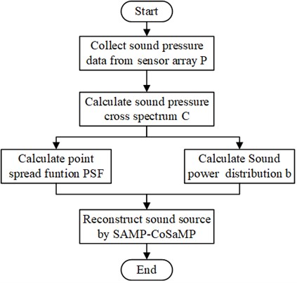
Deconvolution beamforming for sound source imaging is the equation solution process of $b = A x$ . Compressive sensing is a reverse solution process of x, while measurement matrix $Ф$ and observation vector are known. Both relate to the inverse solving of linear functions with two known variables, and compressive sensing provides a variety of reconstruction algorithms for that purpose. Therefore, $b$ and $A$ can be treated as the input of compressive sensing. The original signal can then be restored via the compressive sensing reconstruction algorithm. The proposed SAMP-CoSaMP is further combined with DAMAS. Afterward, an improved beamforming algorithm named SC-DAMAS can be realised for sound source localisation. The principle flow diagram of the SC-DAMAS is depicted in Fig. 1.

Fig. 1Principle flowchart of the improved beamforming algorithm

3. Simulation model building

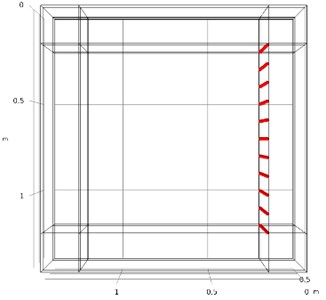
Simulation analysis is performed to demonstrate the effectiveness of SC-DAMAS to address sound source localisation issues. First, a free sound field area with a size of 3×4×3 m in the COMSOL multiphysics simulation environment was constructed. Then, a monopole sound source was set at coordinates of 1.7 m, 3 m, and 1.7 m, from which the volume flow rate is e-3 m³/s. The medium in the entire area was set as air with a relative humidity of 50 %, and the fluid model was set to atmospheric attenuation. To avoid the reflection and absorption of the sound waves propagating to the wall, a perfect matching layer with a thickness of 0.2 m was added to the outside of the area. The measurement surface was placed 1 m away from the sound source surface. On the measurement surface of 1×1 m, the measurement points were 0.1 m apart, and the array of measurement elements was 11×11. To reduce computational work, the local area that contained the sound source and the measurement surface were considered the target areas. The mesh division and schematic diagram of the measuring point of the redefined target area are shown in Fig. 2 and Fig. 3.

Fig. 2Mesh division

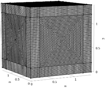
Fig. 3Schematic diagram of measurement array

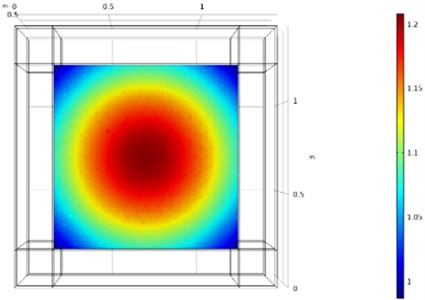
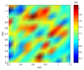
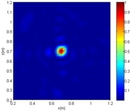
Based on the constructed model, the sound wave in the frequency range of 100 Hz-5000 Hz is simulated with a step length of 100 Hz. The absolute pressure was used as the control pressure. The 2000 Hz simulation results are shown in Fig. 4.

Fig. 4Simulation result of 2000 Hz

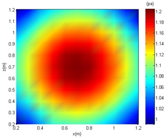
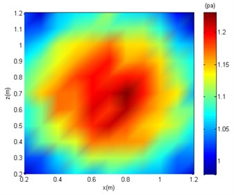
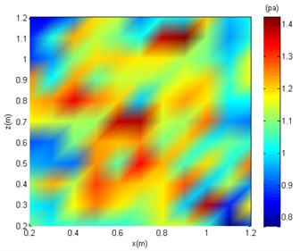
For variable parameter analysis, Gaussian white noise with a signal-to-noise ratio (SNR) equal to 40 dB, 20 dB, and 10 dB was separately added to the sound pressure obtained from the measurement surface. For instance, the simulated surface sound pressure distribution under different SNRs and a sound source frequency of 2000 Hz is shown in Fig. 5.

Fig. 5 shows that the sound pressure on the measurement surface is relatively concentrated under noise-free conditions. On the other hand, further analysis is needed for precise sound source localisation due to the sidelobe. After adding noise (SNR = 40 dB), the aggregation characteristics of the sound pressure field are less clear. Under SNR = 20 dB and SNR = 10 dB, the sound pressure distribution becomes chaotic, and the sound centre cannot be determined. In the following text, SC-DAMAS was applied for sound source localisation with the effects of white noise.

Fig. 5The sound pressure distribution of the measuring surface

a) Noise-free condition

b) SNR = 40 dB

c) SNR = 20 dB

d) SNR = 10 dB

4. Results analysis

4.1. Evaluation of the SAMP-CoSaMP algorithm

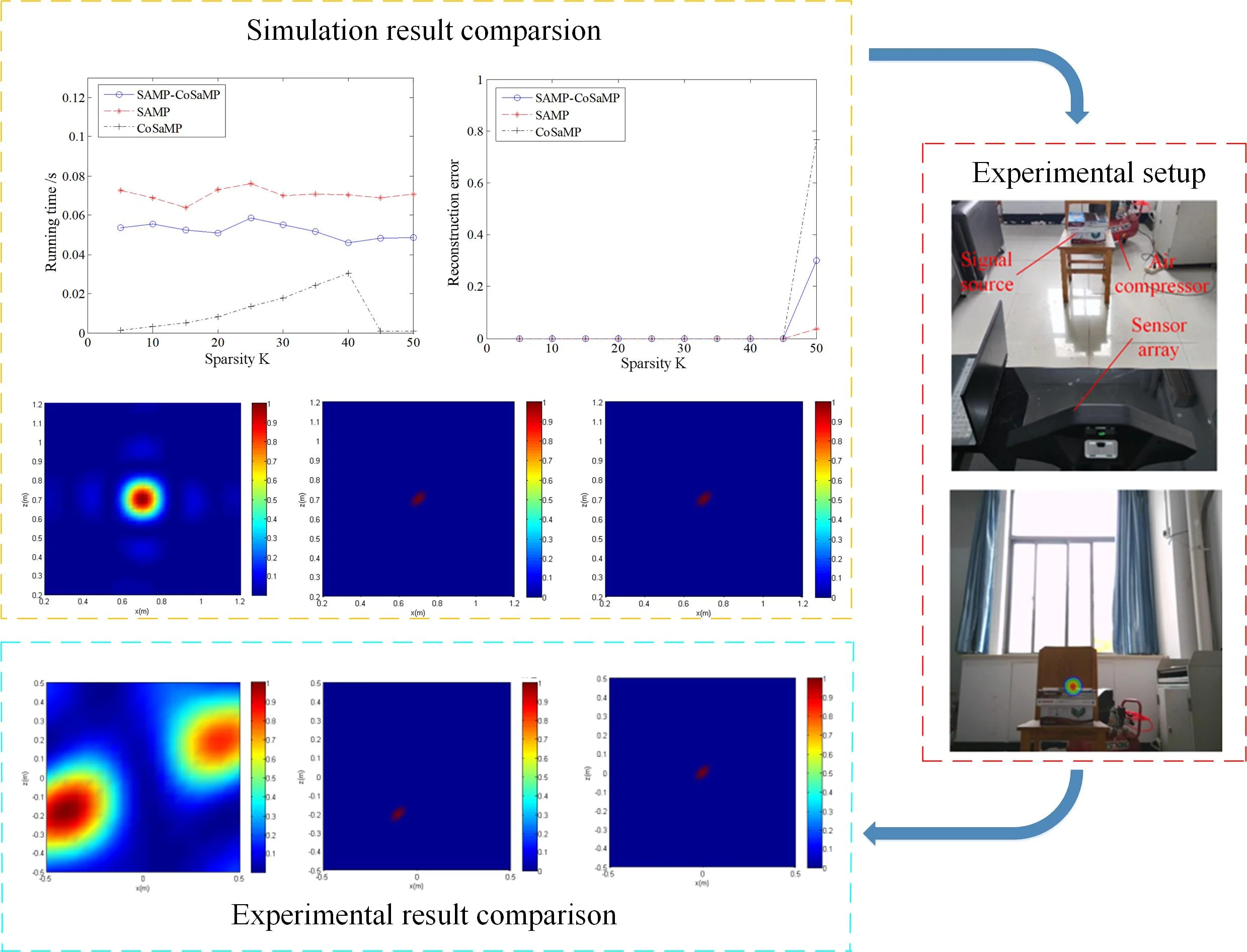
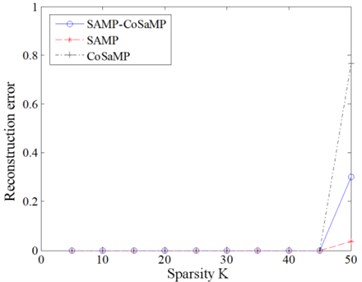
First, to intuitively evaluate the reconstruction performance of SAMP-CoSaMP, relative comparative simulations with those of SAMP and CoSaMP were performed. Assume that there is a sparse signal, the number of measurement points is 128, and the signal length is 512. In the case of a noise-free environment and SNR = 20 dB, the three algorithms are employed for reconstruction, and each group of experiments is repeated 100 times and averaged using the Monte Carlo method. The running time and reconstruction error of each algorithm under variable sparsity are provided in Fig. 6 and Fig. 7.

Fig. 6Simulation result of noise-free

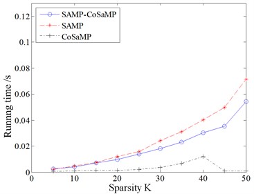
a) Running time

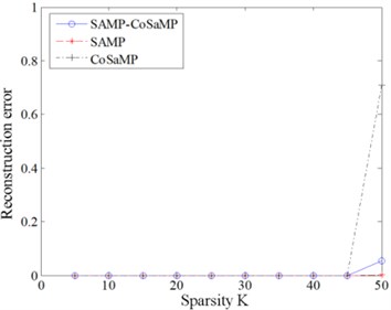
b) Reconstruction error

Fig. 7Simulation result of SNR = 20 dB

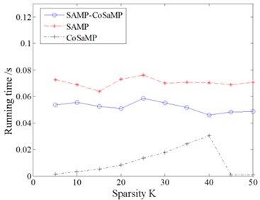
a) Running time

b) Reconstruction error

Fig. 6 and Fig. 7 shows that the SAMP algorithm has the longest running time under the same sparsity. SAMP-CoSaMP has the next longest running time, and then CoSaMP has the shortest running time. Regarding the reconstruction error, a clear sparsity threshold ( $K =$ 45) exists. Within the sparsity threshold, the reconstruction errors of all three algorithms are consistent and negligible (less than 0.01). Otherwise, when $K >$ 45, the reconstruction error of each algorithm will rise rapidly with respect to sparsity, and the average reconstruction error follows the sequence CoSaMP > SAMP-CoSaMP > SAMP. In summary, except for the adaptive characteristic to sparsity, the proposed SAMP-CoSaMP achieves a respectable tradeoff between fast running and reconstruction error.

4.2. Simulation of sound source localisation

In a practical environment, the target sound source signal could be submerged by noise, especially for low SNR cases, which negatively affects the information extraction and imaging of the target sound source. Therefore, sound source localisation issues under low SNR conditions are prioritised in engineering practice. In this study, the conventional beamforming method (CBF), orthogonal matching pursuit algorithm-based deconvolution approach (OMP-DAMAS), and SC-DAMAS are used to process the measured sound field data of different frequencies. First, to analyse efficiency, the three algorithms are individually run 10 times in different frequency scenarios. The average running times are listed in Table 1.

Table 1Running time of the three algorithms

Algorithm	1000 Hz	2000 Hz	4000 Hz
CBF	0.52 s	0.54 s	0.54 s
OMP-DAMAS	2.15 s	2.18 s	2.22 s
SC-DAMAS	2.41 s	2.29 s	2.26 s

Table 1 shows that the sound frequency does not clearly affect the running time of the three algorithms. Under different frequencies, CBF has the shortest running time, and SC-DAMAS has the longest running time, which can be explained by the fact that the SC-DAMAS algorithm must search for the sparsity value. However, the duration of each algorithm is still within the acceptable range. More detailed sound pressure distribution from the simulation is shown in Fig. 8, Fig 9, and Fig. 10.

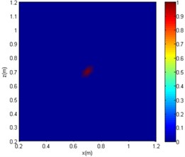
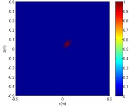
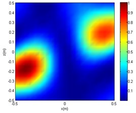
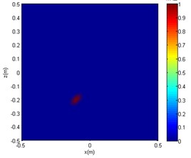
The centre coordinates of the sound source by the three algorithms are (0.7 m, 0.7 m). Although all of the algorithms can be used for sound source localisation, the CBF and OMP-DAMAS methods still have certain defects. More specifically, the imaging size of CBF is greatly affected by sound frequency, since the sidelobe becomes large as sound frequency decreases. In other words, a large source localisation error could be introduced by CBF for low-frequency sound. The OMP-DAMAS method has decent performance in a wide frequency range without sidelobe interference. However, the sparsity must be entered as a necessary parameter for the function solution, which limits its wide application in practice, as the number of sound sources is generally unknown before sound source localisation. SC-DAMAS is an adaptive method in which the sparsity does not need to be determined in advance. Moreover, its imaging results are similar to those of OMP-DAMAS in a wider frequency range, featuring strong robustness and high quality sound source localisation without clear sidelobes. The characteristics of the three methods for sound source localisation are summarised in Table 2.

Fig. 8The imaging comparison of f= 1000 Hz

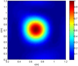
a) CBF

b) OMP-DAMAS

c) SC-DAMAS

Fig. 9The imaging comparison of f= 2000 Hz

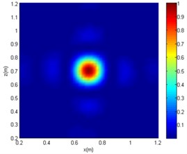
a) CBF

b) OMP-DAMAS

c) SC-DAMAS

Fig. 10The imaging comparison of f= 4000 Hz

a) CBF

b) OMP-DAMAS

c) SC-DAMAS

Table 2Comparison of imaging results

Algorithm	Sidelobe	Predetermined K	Suitable frequency
CBF	Clear	No	High
OMP-DAMAS	Unclear	Yes	Wide
SC-DAMAS	Unclear	No	Wide

5. Validation of SC-DAMAS

To verify the effectiveness of the proposed SC-DAMAS in an actual low SNR environment, a sound source locaiation experiment is conducted. The workshop, standard signal source noise, and air compressor noise are employed as the experimental site, research object, and background noise, respectively. Before the experiment, the sound pressure level of the standard signal source and the working noise of the air compressor were measured to determine the SNR of the entire experimental environment. During the experiment, sound waves with frequencies of 1200 Hz and 2800 Hz are generated successively by an HD1910 standard signal generator, and its sound pressure level is maximised. In that case, the obtained sound pressure level is recorded as 69.2 dB. Afterwards, the signal generator was turned off and the air compressor was turned on. The sound pressure level was measured to be 74.8 dB.

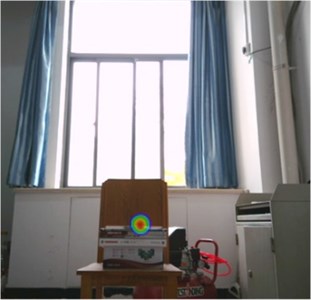
In the experimental measurement, the signal generator and the centre of the sensor array are placed on the same horizontal line, and the distance between the two is 1.5 m horizontally and 1.1 m vertically above the ground. Therefore, the real centre of the sound source in the sensor array is (0,0). The signal generator and the air compressor are turned on simultaneously. Next, the sound array device is turned on to start collecting sound data. The location of the experimental setup and imaging result site are shown in Fig. 11 and Fig. 12. After the experiment, the measured real-time sound pressure data by the sound array are exported to the host computer, the sound pressure collected under the stable sound field is selected as the input, and the CBF, OMP-DAMAS, and SC-DAMAS algorithms are adopted to perform sound source imaging at 1200 Hz and 2800 Hz. The imaging results are shown in Fig. 13, Fig. 14, and Table 3.

Table 3Comparative sound source localisation results

Frequency	1200 Hz	2800 Hz
CBF	(–0.5 m, 0.25 m)	(–0.4 m, 0.2 m)
CBF	(0.5 m, 0.25 m)	(0.4 m, 0.25 m)
OMP-DAMS	(0.11 m, 0.18 m)	(–0.1 m, 0.2 m)
SC-DAMAS	(0.05 m, 0.05 m)	(0, 0)

Fig. 11Experimental setup

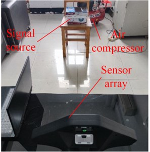
Fig. 12Experimental result

Figs. 13 and 14 show that under the same SNR and sound frequency, the CBF imaging results are severely distorted. It failed to locate the sound source, as another sound source of interference was generated. The OMP-DAMAS method does not show other sources of interference and also cannot correctly locate the location of the noise source. According to Table 3, large localisation errors exist in OMP-DAMAS for the experimental data. The imaging results of the SC-DAMAS method have certain errors but the number of errors are within the acceptable range. In summary, under the conditions of the same SNR and different sound source frequencies, clear sidelobes, as well as disturbing sound centres, emerge in the sound source imaging of CBF. Although the OMP-DAMAS algorithm does not have the problem of having sidelobes, the sound source localisation error is large due to background noise. The imaging of the SC-DAMAS method will not create clear sidelobes and has high localisation accuracy. Therefore, the applicability of the reported algorithm for sound source localisation of low SNR is verified.

Fig. 13The experimental imaging comparison of f= 1200 Hz

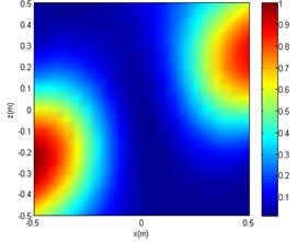
a) CBF

b) OMP-DAMAS

c) SC-DAMAS

Fig. 14The experimental imaging comparison of f= 2800 Hz

a) CBF

b) OMP-DAMAS

c) SC-DAMAS

6. Conclusions

In this study, a novel deconvolution beamforming method is derived for addressing the sound source localisation issue of a low SNR. For its adaptive feature, a hybrid compressive sensing reconstruction algorithm called SAMP-CoSaMP is proposed first. Multiple comparative simulations demonstrate that the hybrid algorithm not only eliminates the dependence of the original CoSaMP on the sparsity but also reduces the SAMPS’s inefficiency. Specifically, the algorithm efficiency is CoSaMP > SAMP-CoSaMP > SAMP, and the algorithm reconstruction error is SAMP > SAMP-CoSaMP > CoSaMP. Then, the adaptive sound source localisation approach is combined with DAMAS and termed SC-DAMAS. Its sound source imaging has a smaller sidelobe than the CBF algorithm in the low frequency range. In addition, it overcomes the limitation that the sparsity value must be preset when using the OMP-DAMAS technique. In summary, SC-DAMAS creates a decent tradeoff between operating efficiency and sound source imaging error. It can be used to address the localisation issue of sound sources with low SNRs over a wide frequency range, especially when the number of sound sources is unknown.

References

P. Chiariotti, M. Martarelli, and P. Castellini, “Acoustic beamforming for noise source localization – Reviews, methodology and applications,” Mechanical Systems and Signal Processing, Vol. 120, pp. 422–448, Apr. 2019, https://doi.org/10.1016/j.ymssp.2018.09.019

Publisher
D. Sun, C. Ma, J. Mei, and W. Shi, “Improving the resolution of underwater acoustic image measurement by deconvolution,” Applied Acoustics, Vol. 165, p. 107292, Aug. 2020, https://doi.org/10.1016/j.apacoust.2020.107292

Publisher
X. Huang, “Compressive sensing and reconstruction in measurements with an aerospace application,” AIAA Journal, Vol. 51, No. 4, pp. 1011–1016, Apr. 2013, https://doi.org/10.2514/1.j052227

Publisher
D. L. Donoho, “Compressed sensing,” IEEE Transactions on Information Theory, Vol. 52, No. 4, pp. 1289–1306, Apr. 2006, https://doi.org/10.1109/tit.2006.871582

Publisher
E. Sejdić, I. Orović, and S. Stanković, “Compressive sensing meets time-frequency: An overview of recent advances in time-frequency processing of sparse signals,” Digital Signal Processing, Vol. 77, pp. 22–35, Jun. 2018, https://doi.org/10.1016/j.dsp.2017.07.016

Publisher
P. K. T. Wu, N. Epain, and C. Jin, “A dereverberation algorithm for spherical microphone arrays using compressed sensing techniques,” in ICASSP 2012 – 2012 IEEE International Conference on Acoustics, Speech and Signal Processing, pp. 4053–4056, Mar. 2012, https://doi.org/10.1109/icassp.2012.6288808

Publisher
L. Wang, Y. Liu, L. Zhao, Q. Wang, X. Zeng, and K. Chen, “Acoustic source localization in strong reverberant environment by parametric Bayesian dictionary learning,” Signal Processing, Vol. 143, pp. 232–240, Feb. 2018, https://doi.org/10.1016/j.sigpro.2017.09.005

Publisher
S. K. Sahoo and A. Makur, “Signal recovery from random measurements via extended orthogonal matching pursuit,” IEEE Transactions on Signal Processing, Vol. 63, No. 10, pp. 2572–2581, May 2015, https://doi.org/10.1109/tsp.2015.2413384

Publisher
D. Needell and R. Vershynin, “Signal recovery from incomplete and inaccurate measurements via regularized orthogonal matching pursuit,” IEEE Journal of Selected Topics in Signal Processing, Vol. 4, No. 2, pp. 310–316, Apr. 2010, https://doi.org/10.1109/jstsp.2010.2042412

Publisher
M. A. Davenport, D. Needell, and M. B. Wakin, “Signal space CoSaMP for sparse recovery with redundant dictionaries,” IEEE Transactions on Information Theory, Vol. 59, No. 10, pp. 6820–6829, Oct. 2013, https://doi.org/10.1109/tit.2013.2273491

Publisher
S. Bonettini, M. Prato, and S. Rebegoldi, “A block coordinate variable metric linesearch based proximal gradient method,” Computational Optimization and Applications, Vol. 71, No. 1, pp. 5–52, Sep. 2018, https://doi.org/10.1007/s10589-018-0011-5

Publisher
N. Nguyen, D. Needell, and T. Woolf, “Linear convergence of stochastic iterative greedy algorithms with sparse constraints,” IEEE Transactions on Information Theory, Vol. 63, No. 11, pp. 6869–6895, Nov. 2017, https://doi.org/10.1109/tit.2017.2749330

Publisher
T. D. Thong, G. Lu, N. Nguyen, and D. T. Trac, “Sparsity adaptive matching pursuit algorithm for practical compressed sensing,” in Conference on Signals, Systems and Computers, 2010.

Search CrossRef
W. Ma and X. Liu, “Compression computational grid based on functional beamforming for acoustic source localization,” Applied Acoustics, Vol. 134, pp. 75–87, May 2018, https://doi.org/10.1016/j.apacoust.2018.01.006

Publisher
E. Sarradj, “A fast signal subspace approach for the determination of absolute levels from phased microphone array measurements,” Journal of Sound and Vibration, Vol. 329, No. 9, pp. 1553–1569, Apr. 2010, https://doi.org/10.1016/j.jsv.2009.11.009

Publisher
Riccardo Zamponi, Nicolas van de Wyer, and Christophe Schram, “An improved regularization of the generalized inverse beamforming applied to a benchmark database,” in BeBeC 2018, Mar. 2018.

Publisher
J. Wang and W. Ma, “Deconvolution algorithms of phased microphone arrays for the mapping of acoustic sources in an airframe test,” Applied Acoustics, Vol. 164, p. 107283, Jul. 2020, https://doi.org/10.1016/j.apacoust.2020.107283

Publisher
J. A. Högbom, “Aperture synthesis with a non-regular distribution of interferometer baselines,” Astronomy and Astrophysics Supplement Series, Vol. 15, p. 417, Jun. 1974.

Search CrossRef
P. Sijtsma, “CLEAN based on spatial source coherence,” International Journal of Aeroacoustics, Vol. 6, No. 4, pp. 357–374, Dec. 2007, https://doi.org/10.1260/147547207783359459

Publisher
T. F. Brooks and W. M. Humphreys, “A deconvolution approach for the mapping of acoustic sources (DAMAS) determined from phased microphone arrays,” Journal of Sound and Vibration, Vol. 294, No. 4-5, pp. 856–879, Jul. 2006, https://doi.org/10.1016/j.jsv.2005.12.046

Publisher
K. Ehrenfried and L. Koop, “Comparison of iterative deconvolution algorithms for the mapping of acoustic sources,” AIAA Journal, Vol. 45, No. 7, pp. 1584–1595, Jul. 2007, https://doi.org/10.2514/1.26320

Publisher
O. Lylloff, E. Fernández-Grande, F. Agerkvist, J. Hald, E. Tiana Roig, and M. S. Andersen, “Improving the efficiency of deconvolution algorithms for sound source localization,” The Journal of the Acoustical Society of America, Vol. 138, No. 1, pp. 172–180, Jul. 2015, https://doi.org/10.1121/1.4922516

Publisher

Cited by

Proceedings of International Conference on Artificial Intelligence and Communication Technologies (ICAICT 2023)

Kewen Wang | Yu Wu | Jiawei Tian

(2024)

An improved deconvolution beamforming algorithm for acoustic imaging of low signal-to-noise ratio sound sources in reverberant field

Wenyong Guo | Hantao Chen | Jing Xia | Xiaofeng Li | Chenghao Cao

(2023)

About this article

Received

02 October 2021

Accepted

12 January 2022

Published

15 May 2022

SUBJECTS

Acoustics, noise control and engineering applications

DOI

https://doi.org/10.21595/jve.2022.22232

Keywords

beamforming algorithm

sound source localization

compressive sensing

Sparsity

This is an open access article distributed under the Creative Commons Attribution License, which permits unrestricted use, distribution, and reproduction in any medium, provided the original work is properly cited.

Previous article in issue Previous Next article in issue Next

Research article

2023 02 09

An improved deconvolution beamforming algorithm for acoustic imaging of low signal-to-noise ratio sound sources in reverberant field

Wenyong Guo, Hantao Chen, Jing Xia, Xiaofeng Li, Chenghao Cao

Research article

2022 06 13

A deconvolution sound source identification method based on twice weak selection orthogonal matching pursuit

Weipeng Zhao, Jin Mao, Kai Liu

Research article

2019 12 31

Source localization in reverberation environment based on improved equivalent sound source near-field acoustic holography algorithm

Hongyu Zhang, Wenyong Guo, Jianggui Han, Hantao Chen

Research article

2018 09 24

The coherent sound field separation method combining compressive sensing

Chen Hantao, Guo Wenyong, Zhang Hongyu

W. Guo, J. Han, H. Chen, L. Yu, and Z. Wu, “An adaptive beamforming algorithm for sound source localisation via hybrid compressive sensing reconstruction,” Journal of Vibroengineering, Vol. 24, No. 3, pp. 591–603, May 2022, https://doi.org/10.21595/jve.2022.22232

Copy Extrica

Copied to clipboard!

TY  - JOUR
DO  - 10.21595/jve.2022.22232
UR  - https://doi.org/10.21595/jve.2022.22232
TI  - An adaptive beamforming algorithm for sound source localisation via hybrid compressive sensing reconstruction
T2  - Journal of Vibroengineering
AU  - Guo, Wenyong
AU  - Han, Jianggui
AU  - Chen, Hantao
AU  - Yu, Li
AU  - Wu, Zhe
PY  - 2022
DA  - 2022/03/17
PB  - JVE International Ltd.
SP  - 591-603
SN  - 1392-8716
SN  - 2538-8460
ER  - 

Copy Ris

Copied to clipboard!

@article{Guo_2022,
	doi = {10.21595/jve.2022.22232},
	url = {https://doi.org/10.21595/jve.2022.22232},
	year = 2022,
	month = {mar},
	publisher = {{JVE} International Ltd.},
	pages = {591--603},
	author = {Wenyong Guo and Jianggui Han and Hantao Chen and Li Yu and Zhe Wu},
	title = {An adaptive beamforming algorithm for sound source localisation via hybrid compressive sensing reconstruction},
	journal = {Journal of Vibroengineering}
}

Copy Bibtex

Copied to clipboard!

[1]W. Guo, J. Han, H. Chen, L. Yu, and Z. Wu, “An adaptive beamforming algorithm for sound source localisation via hybrid compressive sensing reconstruction,” Journal of Vibroengineering, pp. 591–603, Mar. 2022, doi: 10.21595/jve.2022.22232.

Copy IEEE

Copied to clipboard!

Guo, Wenyong, Jianggui Han, Hantao Chen, Li Yu, and Zhe Wu. “An Adaptive Beamforming Algorithm for Sound Source Localisation via Hybrid Compressive Sensing Reconstruction.” Journal of Vibroengineering, March 17, 2022, 591–603. https://doi.org/10.21595/jve.2022.22232.

Copy Chicago

Copied to clipboard!

An adaptive beamforming algorithm for sound source localisation via hybrid compressive sensing reconstruction

Abstract

Highlights

1. Introduction

2. Material and methods

2.1. Preliminary analysis of DAMAS

2.2. SAMP-CoSaMP reconstruction algorithm

2.3. SC-DAMAS algorithm

3. Simulation model building

4. Results analysis

4.1. Evaluation of the SAMP-CoSaMP algorithm

4.2. Simulation of sound source localisation

5. Validation of SC-DAMAS

6. Conclusions

References

Cited by

About this article

Related Articles