Abstract
A traceable reduced-order design workflow is developed for a 13.85 kg lift-plus-cruise vertical take-off and landing (VTOL) unmanned aerial vehicle (UAV). The novelty is a verification architecture – not a new lifting-line relation – that couples archived-data reconciliation, flight-envelope falsification, bounded uncertainty and exact load closure in one reduced-order chain. Thin-airfoil theory and a 20-term Prandtl lifting-line solution are coupled with a bounded parasite-drag scenario, an explicit stall-margin feasibility index, and force-conserving reconstruction of distributed lift, shear force and bending moment. A legacy circulation dataset is an unpublished higher-fidelity numerical distribution retained in the authors’ design archive. Because its original solver settings, speed, density and dimensional force scaling cannot be recovered, it is treated as the available full-order model (FOM) benchmark only for integral-normalized spanwise-shape comparison, not as physical validation. The model predicts a zero-lift angle of –1.92°, a finite-wing lift-curve slope of 0.0903 deg-1 and a span efficiency factor of 0.977. The nominal maximum lift-to-drag ratio is 16.5, with a bounded scenario range of 15.2-18.2. Relative to the archived benchmark, the reduced-order model (ROM) gives an RMSE of 0.1215, a range-normalized RMSE of 10.1 % and a maximum pointwise normalized deviation of 21.2 % for circulation shape. These are shape errors only and do not establish the absolute accuracy of lift, drag or load magnitudes. Most importantly, the archived 36 km/h wing-borne condition is falsified because it requires lift coefficients of 3.89 at sea level and 5.24 at 3000 m. At 3000 m, even 90 km/h is only statically feasible and does not retain the selected 30 % stall-speed margin; the protected minimum is 97.8 km/h. At a design load factor of 2.5, the reconstructed half-wing root shear and bending moment are 169.8 N and 91.9 N·m. The workflow therefore provides a reproducible screening and load-transfer baseline while explicitly identifying the experiments required for physical validation.
1. Introduction
During horizontal flight, the lift-plus-cruise vertical take-off and landing unmanned aerial vehicle (VTOL UAV) uses its wing for lift while the vertical-lift rotors, booms and nacelles remain on board. This gives a runway-independent vehicle without surrendering fixed-wing cruise efficiency, a useful combination for urgent freight, inspection and emergency logistics. The configuration also couples quantities that are often treated separately: the inactive lift installation adds mass and drag, local rotor and boom geometry modifies the wing flow, and the lift coefficient required at a given speed rises as air density decreases. Geometry, atmosphere and load normalization must therefore be closed before aerodynamic performance is compared [1-4]. The same closed aerodynamic state is required by battery-range and electric-propulsion calculations [5], [6]. Recent energy-optimal low-altitude UAV delivery research likewise shows that routing decisions depend on physically credible energy and flight envelopes [7].
For the chord and operating speeds of small UAVs, Reynolds numbers of only a few hundred thousand are typical. In this regime, transition, laminar-separation bubbles and surface finish can change both profile drag and maximum lift appreciably [8-11]. Wind-tunnel measurements are required for physical validation, while higher-fidelity CFD is required to assess omitted flow physics; neither should be conflated with numerical convergence of the reduced-order equations. A reduced-order model remains useful during preliminary design because its governing balances can be inspected, parameter variations are inexpensive, and subsequent CFD or experiments can be compared with a traceable baseline [12-15].
In this study, the main difficulty was not solver selection but reconciliation of the available design records. The archive contained usable CAD views, numerical distributions and solver images, yet span, mass, airfoil and density values were not uniform between records. Combining them without correction would produce coefficients referenced to different geometries or atmospheric states, and a spanwise distribution that might not recover the prescribed lift. The calculation chain was therefore built only after dimensional consistency, reference area, atmospheric state and integral load closure had been checked.
The relation between this work and the authors’ earlier publications is limited and explicit. Reference [16] describes the wider platform family and a NACA 4412 CFD case at 35 m/s; here, only its full-configuration drag level is used as prior calibration evidence. The present calculations use the confirmed 2.62 m-span NACA 2312 wing. Reference [17] documents the platform’s geometric lineage, while [18] is cited only in relation to manufacturing-induced geometric deviations. None of the earlier coefficient distributions is reported as a result of the current model.
The novelty is not the Prandtl solver, thin-airfoil relation, standard atmosphere or spanwise integration individually. It is the auditable verification architecture that closes inconsistent archived inputs and applies two explicit falsification gates: integral force conservation and a protected-flight feasibility index. The workflow first reduces conflicting records to one parameter set; couples altitude-dependent Reynolds effects to lifting-line and drag calculations; separates static lift balance from a selected operational margin; quantifies reduced-order/full-order circulation-shape discrepancy; and reconstructs lift, shear and bending without changing total force. The archived 36 km/h requirement is then tested rather than assumed and is rejected when it demands an unattainable lift coefficient. This combination of traceability, falsification and exact load transfer is the study’s specific contribution to preliminary transport-UAV design and to mathematical modelling of engineering systems.
2. Research object and consistency closure
2.1. Lift-plus-cruise configuration
The aircraft considered here has a swept, tapered wing blended into a centrebody, four lift propellers on two booms, and a separate cruise propulsor. During wing-borne flight the lift assembly remains installed and contributes mass and interference drag. Fig. 1 combines the front, top, isometric and rear/top CAD views used to establish configuration topology and reference dimensions. These archive views support the geometry audit but are not used as a watertight CFD surface.
The canonical wing has span 2.62 m, reference area 0.57 m2 and mass 13.85 kg. The root and tip chords reconstructed from the tabulated planform are 0.3403 and 0.1001 m. The resulting taper ratio is 0.294, aspect ratio 12.04 and mean aerodynamic chord 0.242 m. These quantities are mutually compatible to engineering accuracy. The alternative span of 2.0 m, mass of 12 kg and sea-level density appearing in intermediate records are excluded from the computational chain because mixing them would change wing loading, Reynolds number and required lift simultaneously.
Fig. 1Canonical lift-plus-cruise VTOL UAV configuration reconstructed from the authors’ CAD archive: a) front view; b) top view; c) isometric view; d) rear/top view. Source: authors’ original computer-generated CAD archive; this figure is not a photograph and contains no third-party or identifiable-person content

a) Front view
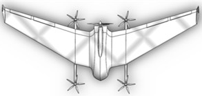
b) Top view
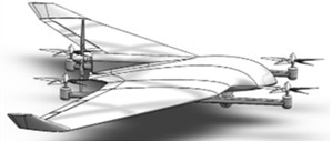
c) Isometric view
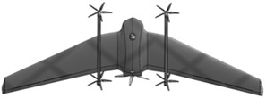
d) Rear/top view
Table 1Canonical geometric and operational parameters used in every model
Parameter | Symbol | Value | Unit / note |
Take-off mass | 13.85 | kg | |
Wing span | 2.62 | m | |
Reference wing area | 0.57 | m2 | |
Root / tip chord | 0.3403 / 0.1001 | m | |
Taper ratio | 0.294 | – | |
Aspect ratio | AR | 12.04 | b2/S |
Mean aerodynamic chord | 0.242 | m | |
Wing loading | 238.4 | N/m2 | |
Airfoil | – | NACA 2312 | 0.02, 0.30, 0.12 |
Declared cruise interval | 70-90 | km/h | |
Altitude interval | 0-3000 | m |
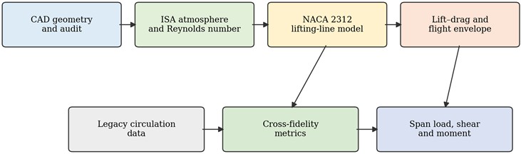
Fig. 2 shows the order applied to every evaluated condition. The CAD-derived parameter record first fixes geometry and atmosphere; aerodynamic coefficients are then calculated; the legacy circulation data are introduced only for comparison; and internal loads are recovered only after total force has been imposed. Keeping these stages separate avoids using a derived quantity as if it were independent validation data.
Fig. 2Computational workflow linking the canonical CAD geometry, reduced-order model, legacy distribution and load reconstruction
2.2. Geometric and atmospheric closure
For a linearly tapered wing, chord, taper ratio, aspect ratio and mean aerodynamic chord are closed by Eq. (1). The span coordinate y is measured from the symmetry plane and . The reference area is kept at the confirmed CAD value rather than recomputed from rounded chord values; this avoids allowing presentation rounding to modify the force normalization:
Atmospheric temperature, pressure and density are obtained together from the tropospheric International Standard Atmosphere [19]. Dynamic viscosity follows Sutherland’s relation, and the local sound speed is evaluated for the Mach-number check. Calculating this set from one altitude prevents accidental use of sea-level density in the 3 km aerodynamic state:
At 3000 m, Eq. (2) gives 268.66 K and 0.909 kg/m³. For 70-90 km/h, Eq. (3) gives 2.52×10⁵-3.25×10⁵ and 0.060-0.077. Compressibility is therefore negligible, but low-Reynolds-number effects cannot be ignored in the drag and stall uncertainty. The often-repeated value 0.092 kg/m3 is rejected as a decimal-place error: it would imply an altitude far outside the stated mission and inflate the required lift coefficient by nearly one order of magnitude.
3. Mathematical aerodynamic model
3.1. NACA 2312 section and zero-lift incidence
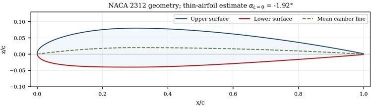
The analytical four-digit NACA definition was chosen so that the section can be regenerated without an external coordinate file. For NACA 2312, the maximum camber, its chordwise location and maximum thickness are 2 %, 30 % and 12 % of chord, respectively. Eq. (4) gives the piecewise mean-camber line and slope in the normalized coordinate /:
Thin-airfoil theory is used only to determine the zero-lift reference, not to predict viscous profile drag. With , the section zero-lift angle follows from the weighted camber-line slope. Numerical quadrature of Eq. (5) gives –1.918°, which explains the positive lift at zero geometric incidence:
Fig. 3NACA 2312 section generated from the analytical four-digit definition
3.2. Finite-wing lifting-line solution
The wing is represented by Prandtl’s circulation series with odd harmonics, which enforces symmetry while allowing a non-elliptic tapered loading. Twenty terms are used; increasing the system to 30 terms changes and by less than 0.15 % over the pre-stall range. At each collocation point , the unknown Fourier coefficients are obtained from Eq. (6). A two-dimensional lift slope 0.95(2)rad-1 is adopted to avoid applying an inviscid 2 value without allowance for the Reynolds regime. The 5 % reduction is treated as a model-form assumption in the sensitivity study:
After solution of the collocation system, Eq. (7) gives total lift, induced drag and span efficiency. Airspeed sets the circulation magnitude, whereas planform and effective incidence govern its normalized spanwise form. The latter property permits one circulation shape to be rescaled to a prescribed aircraft load without changing the integral force:
3.3. Parasite drag and force coefficients
Conceptual wing methods do not resolve boom, motor and centrebody interference. The total drag polar is therefore written as the sum of a system-level parasite term and lifting-line induced drag. The nominal zero-lift parasite-drag coefficient of 0.034 is transferred from the authors’ earlier NACA 4412 full-configuration CFD point after induced drag is removed [16]. The ±0.006 band is not a statistical confidence interval. It is a deliberately symmetric engineering scenario spanning 0.028-0.040, or ±17.6 % of the nominal value, to expose sensitivity to the changed airfoil, Reynolds number, surface finish and unresolved configuration interference documented as important at low Reynolds number [8-11]. Consequently, the resulting lift-to-drag interval is interpreted as a bounded scenario result rather than a validated uncertainty distribution:
Lift and drag are dimensionalized with the same density, speed and full-planform reference area used to define the coefficients. This is necessary for the cross-fidelity comparison: substituting wetted area, half-wing area or sea-level density at a later stage would change the force scale while leaving the coefficient unchanged:
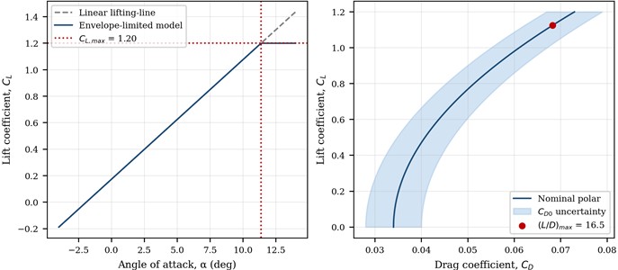
Fig. 4Reduced-order lift curve and calibrated drag polar; shaded drag interval represents model-form uncertainty in non-lifting components
3.4. Flight-envelope feasibility
The aerodynamic model is connected to transport operation by calculating the lift coefficient required for level flight. A condition can satisfy and still be operationally weak because it lies too close to stall. The protected design limit is therefore written in speed form, using a prescribed speed margin 1.30:
For mapping purposes, Eq. (11) defines a dimensionless feasibility index . Values 1 meet the selected 30 % speed margin; 1 may sustain ideal level flight but do not retain that margin; smaller values are infeasible even before manoeuvre or gust loads are added. This distinction prevents the label “feasible” from being applied to a near-stall cruise point.
The multiplier of 1.30 is an explicit preliminary-design screening choice, not a certification claim. Current FAA Part 23 requires structural design airspeeds to remain sufficiently above stall to protect against loss of control in turbulence and to provide practical operational limits [20], but it does not convert the present analytical index into a compliance demonstration. Applicable unmanned-aircraft requirements, calibrated stall data and flight tests are still required:
3.5. Load-conserving spanwise reconstruction
The circulation series is transformed into an aerodynamic load shape. Instead of using an arbitrary dimensional multiplier, the shape is normalized so that the two half-wings carry the prescribed total load . This removes the unit inconsistency found when mass in kilograms is inserted directly into a force balance:
The internal shear and bending moment at a station y are obtained by integration toward the tip. The derivatives satisfy and ; time t is not involved. Eq. (14) is valid for the clean aerodynamic wing load. Concentrated boom, motor, battery and landing loads must be superposed at their measured stations in a detailed structural model and are intentionally not invented here:
4. Numerical experiment and cross-fidelity comparison protocol
4.1. Computational chain
Each numerical-experiment case follows the sequence in Fig. 2 with a single immutable parameter record. Thus, a change in altitude, reference area or mass propagates through aerodynamics, feasibility and structural loading rather than only one branch of the calculation. The script stores unrounded values and applies rounding only when tables are generated, so the reported cases can be reproduced without commercial software.
Table 2Numerical-experiment matrix and numerical settings
Group | Setting | Values |
Geometry | Planform / section | Tapered wing; NACA 2312 |
Atmosphere | Altitude h | 0, 1000, 2000 and 3000 m |
Transport condition | True airspeed V | 36 and 70–115 km/h |
Aerodynamic sweep | Angle of attack α | −4° to 14°; 0.2° increment |
Lifting-line | Series order N | 20 odd harmonics |
Span integration | Semi-span stations | 1601 uniform points |
Design constraints | 1.20 / 1.30 / 1.0 and 2.5 | |
Uncertainty cases | ±5 % / ±0.006 / ±0.10 |
4.2. Legacy numerical-data provenance and conditioning
The comparison dataset is an unpublished higher-fidelity numerical circulation distribution retained in the authors’ earlier internal design archive. For the requested reduced-order model (ROM) versus full-order model (FOM) error statement, this archived distribution is treated as the available FOM benchmark solely for a dimensionless shape comparison. Its source table provides dimensionless values at 12 span stations and combines baseline and correction components, but the original solver, mesh, turbulence treatment, speed, density and dimensional force scaling cannot now be recovered consistently. Each curve is therefore divided by its semi-span integral, removing the unknown scale and testing only whether the two distributions place relative load in the same wing regions:
No parameter is fitted to the archived curve. The lifting-line ROM is sampled at the same normalized span stations and evaluated with the canonical planform. The resulting ROM-FOM residuals quantify circulation-shape discrepancy, but they cannot identify a physical cause: they may arise from centrebody or propeller-boom interference, from undocumented assumptions in the archived calculation, or from both.
4.3. Numerical-verification, comparison and uncertainty metrics
Three pointwise shape-comparison measures are reported: RMSE, RMSE normalized by the legacy range, and maximum normalized deviation. They are distinct from the numerical-convergence and force-conservation checks. A separate integral check is retained because close pointwise shape agreement does not guarantee the prescribed total lift. Eq. (16) evaluates the shape metrics at the common span stations:
Uncertainty is examined one parameter at a time for the two-dimensional lift slope, parasite drag and maximum lift. For any output , Eq. (17) expresses the centred response to a fractional change in the selected input. The calculation ranks missing measurements; it does not manufacture a probability distribution from unsupported assumptions. The interpretation follows the established separation between code verification, model comparison, physical validation and uncertainty propagation [21-27]:
5. Results
5.1. Aerodynamic coefficients
The lifting-line solution is linear up to the imposed stall boundary. It gives 0.173 at zero incidence, confirming the effect of NACA 2312 camber, and a finite-wing slope of 0.0903 deg-1.
The predicted span efficiency is 0.977 and is nearly constant in the linear range because all Fourier coefficients scale with effective incidence. This high value is plausible for a smoothly tapered high-aspect-ratio wing, but it should not be interpreted as a full-aircraft efficiency: boom, fuselage and propeller slipstream effects enter uncertainty rather than the clean-wing .
Table 3Predicted aerodynamic coefficients for the NACA 2312 tapered wing
(deg) | / | Model status | |||
–4 | –0.188 | 0.0010 | 0.0350 | –5.4 | Linear |
–2 | –0.007 | 0.0000 | 0.0340 | –0.2 | Linear |
0 | 0.173 | 0.0008 | 0.0348 | 5.0 | Linear |
2 | 0.354 | 0.0034 | 0.0374 | 9.5 | Linear |
4 | 0.534 | 0.0077 | 0.0417 | 12.8 | Linear |
6 | 0.715 | 0.0138 | 0.0478 | 14.9 | Linear |
8 | 0.895 | 0.0217 | 0.0557 | 16.1 | Linear |
10 | 1.076 | 0.0313 | 0.0653 | 16.5 | Linear |
12 | 1.256 | 0.0427 | 0.0730 | 16.4 | Beyond design stall |
The nominal polar reaches its maximum near 1.12, producing 16.5. The optimum lies close to the upper pre-stall region, so uncertainty in and matters more than small changes in lifting-line order. When changes from 0.028 to 0.040, the predicted maximum spans approximately 18.2 to 15.2. This interval is reported instead of a single over-precise efficiency claim.
5.2. Altitude-speed transport envelope
Fig. 5 is the central operational result. The 1 contour moves to higher true airspeed as altitude increases. At sea level, a 30 % stall-speed margin requires 84.3 km/h; at 3000 m it requires 97.8 km/h. The declared 70-90 km/h band therefore contains protected operating points only near the lower part of the altitude envelope. At 3 km, 70 km/h is statically infeasible and 80-90 km/h can support ideal level flight, but neither preserves the selected 30 % margin.
Fig. 5Altitude–speed feasibility map for CL,max= 1.20 and a 30 % stall-speed margin
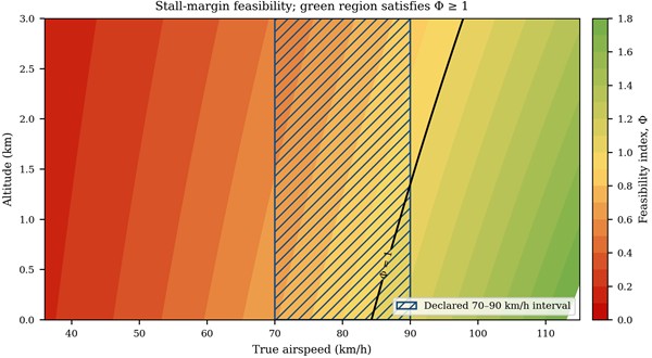
The low-speed value 36 km/h is retained as a falsification test rather than a cruise condition. It requires 3.89 at sea level and 5.24 at 3 km, which is well outside the capability of an unslotted NACA 2312 wing. This finding is valuable because it exposes a mission requirement that cannot be repaired by numerical tuning. Either the aircraft must transition to wing-borne flight at a higher speed, use powered-lift/high-lift devices validated experimentally, or change wing loading.
5.3. Reduced-order/full-order circulation-shape error
Integral normalization gives both curves the same total area, after which their load placement can be compared directly (Fig. 6). Both unload monotonically toward the tip. The analytical curve, however, has its maximum at the root, whereas the archive curve peaks near 0.2 and remains flatter over the middle span.
Table 4Level-flight and protected-margin feasibility in the declared cruise interval
(m) | (kg/m3) | (km/h) | Classification | ||
0 | 1.225 | 70 | 1.029 | 0.690 | Level flight only |
0 | 1.225 | 80 | 0.788 | 0.901 | Level flight only |
0 | 1.225 | 90 | 0.622 | 1.141 | Protected |
1000 | 1.112 | 70 | 1.134 | 0.626 | Level flight only |
1000 | 1.112 | 80 | 0.868 | 0.818 | Level flight only |
1000 | 1.112 | 90 | 0.686 | 1.035 | Protected |
2000 | 1.006 | 70 | 1.252 | 0.567 | Infeasible |
2000 | 1.006 | 80 | 0.959 | 0.741 | Level flight only |
2000 | 1.006 | 90 | 0.758 | 0.937 | Level flight only |
3000 | 0.909 | 70 | 1.386 | 0.512 | Infeasible |
3000 | 0.909 | 80 | 1.062 | 0.669 | Level flight only |
The residual changes sign near 0.4: it is positive over the inner semi-span and negative over most of the remaining span. This ordered pattern identifies where the two numerical descriptions differ, but it does not prove centrebody shielding or propulsion interference. Undocumented legacy-model assumptions provide an equally plausible explanation. Controlled clean-wing, centrebody, boom and propeller-on cases are required before a causal attribution can be made.
Fig. 6Integral-normalized spanwise circulation and reduced-order/full-order residuals relative to the unpublished archived higher-fidelity distribution
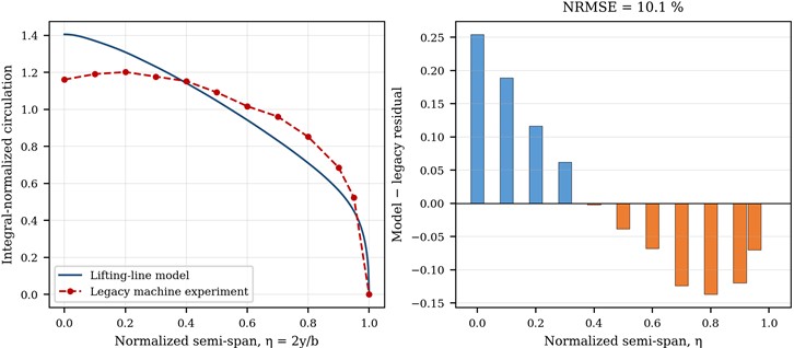
Table 5Reduced-order versus available full-order circulation-shape error metrics
Metric | Value | Interpretation |
Integral of legacy raw curve | 0.9966 | Nearly unit-normalized in the archive |
RMSE | 0.1215 | Pointwise normalized-shape error |
Range-normalized RMSE | 10.1 % | Normalized-shape discrepancy only; not absolute force accuracy |
Maximum normalized deviation | 21.2 % | Located in the inner semi-span |
Lifting-line force closure | < 10⁻⁶ | Numerical integration residual |
With the archived higher-fidelity distribution treated as the available FOM benchmark, the ROM circulation-shape errors are RMSE = 0.1215, range-normalized RMSE = 10.1 % and maximum pointwise normalized deviation = 21.2 %. These values compare two integral-normalized shapes. Because normalization removes amplitude and the benchmark speed, density and dimensional force scale are unavailable, absolute ROM–FOM errors in lift, drag, circulation magnitude and structural-load magnitude cannot be determined from this dataset and are not claimed. The 21.2 % peak local deviation instead identifies the inner semi-span as a priority for controlled RANS calculations or pressure measurements.
5.4. Spanwise shear and bending reconstruction
Eq. (13) closes the total force before the internal loads are integrated. At , each half-wing carries 67.91 N, and the aerodynamic centre of the reconstructed half-wing load lies 0.541 m from the symmetry plane. The corresponding root bending moment is 36.77 N·m. Scaling the same aerodynamic shape to 2.5 gives 169.78 N root shear and 91.91 N·m root bending moment (Fig. 7). The linear scale is exact for the prescribed shape and provides a clean reference load case for a subsequent finite-element model.
Table 6 contains wing aerodynamic reference loads rather than certification limit loads. Wing self-weight, boom and lift-motor inertia, thrust offsets and gust increments must be added once their masses and span stations have been measured. Those data are absent from the design archive, so no assumed point loads were inserted. The reported bending distribution is consequently a traceable baseline for later mass-property measurements and structural combination cases.
Fig. 7Reconstructed distributed lift, shear force and bending moment on one half-wing. Source: authors’ calculations
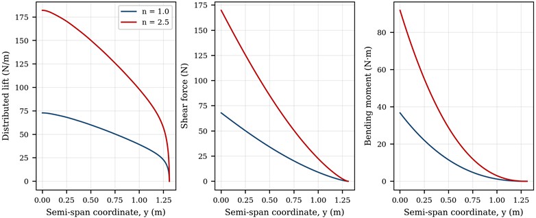
Table 6Integral load-closure results
Load factor | Half-wing lift (N) | Root shear (N) | Root moment (N·m) | Load centroid (m) |
1.0 | 67.91 | 67.91 | 36.77 | 0.541 |
2.5 | 169.78 | 169.78 | 91.91 | 0.541 |
5.5. Design correction and sensitivity
The feasibility map can be inverted to produce an actionable geometry correction. With 3000 m, V = 90 km/h, 1.20 and 1.30, the required area is 0.673 m2, an 18.1 % increase over the current 0.57 m². If geometry is fixed, the minimum protected speed is 97.8 km/h. Fig. 8 shows both alternatives and clarifies that a larger wing is not automatically preferable: area increases skin-friction and structural mass, so the corrected geometry must be returned to the coupled mass-energy design loop.
The ranking shows that must be measured rather than assumed if the aircraft is intended to cruise close to the protected boundary. Parasite drag controls range and efficiency but does not alter level-flight lift closure. Conversely, mass and wing area enter stall speed through a square root; moderate measurement errors have a smaller percentage effect than the uncertainty in low-Reynolds-number maximum lift. The most valuable next experiment is therefore a NACA 2312 wing or full-configuration force sweep through stall at 2.5×10⁵-3.3×10⁵, followed by a limited set of propeller-on interference cases.
Fig. 8Required lift coefficient across altitude and wing-area correction for a 30 % stall-speed margin at 3 km
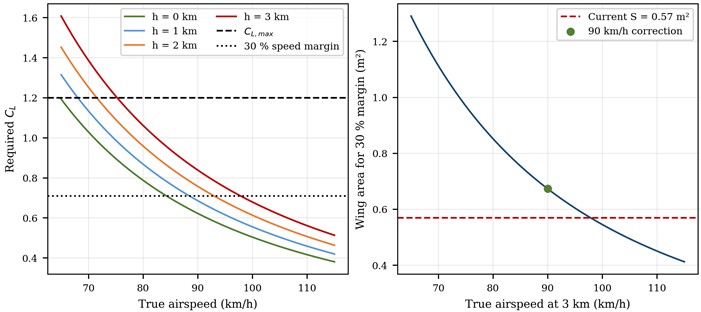
Table 7One-at-a-time sensitivity of principal outputs
Perturbed input | Interval | Dominant output | Observed effect |
Two-dimensional slope | ±5 % | ±4.1 % | |
Parasite drag | 0.028–0.040 | 18.2-15.2 | |
Maximum lift | 1.10–1.30 | at 3 km | 102.2-94.0 km/h |
Mass | ±5 % | at 3 km | ±2.5 % |
Wing area | ±5 % | at 3 km | ∓2.5 % |
5.6. Numerical convergence and conservation
A reduced-order method is useful only when numerical truncation is smaller than physical model-form uncertainty. Two independent code-verification tests were performed. First, the odd lifting-line order was increased from 4 to 40 at 6°. Second, semi-span integration stations increased from 51 to 1601 for the load factor 2.5. Relative change is measured against the most resolved value according to Eq. (18):
Fig. 9Convergence of lifting-line coefficients and reconstructed root bending moment
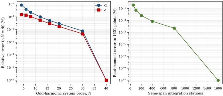
Table 8Numerical-order convergence at the representative aerodynamic and design-load conditions
Discretization | Primary value | Secondary value | Reported quantity |
Lifting-line 4 | 0.720639 | 0.975677 | |
Lifting-line 8 | 0.716092 | 0.976113 | |
Lifting-line 12 | 0.715144 | 0.976614 | |
Lifting-line 20 | 0.714647 | 0.976977 | |
Lifting-line 30 | 0.714491 | 0.977103 | |
Lifting-line 40 | 0.714436 | 0.977148 | |
Load grid | 91.7298 | – | Root M (N·m) |
Load grid | 91.8887 | – | Root M (N·m) |
Load grid | 91.9105 | – | Root M (N·m) |
Load grid | 91.9126 | – | Root M (N·m) |
At the selected order 20, differences from 40 are below 0.01 % for the lift coefficient and 0.02 % for span efficiency. The 1601-station integration changes the root moment by less than 0.01 % relative to 801 stations. These results verify numerical convergence of the implemented reduced-order equations; they do not validate the underlying aerodynamic physics. Their magnitude is two orders smaller than the 10.1 % normalized-shape discrepancy and the parasite-drag scenario range.
Conservation was checked separately from convergence. The normalized load integrates to within 10⁻6 in relative terms, root shear equals one-half of the prescribed aircraft load, and the tip conditions 0 are satisfied by construction. These are verification checks on the numerical implementation, not validation against physical measurements. A future CFD-to-structure transfer should retain the same checks after pressure interpolation so that mapping error cannot create or remove net lift.
6. Discussion
6.1. Scientific contribution and transport-engineering relevance
The scientific contribution is the traceable decision chain between inconsistent design evidence and a conservative transport-flight envelope, not a new lifting-line equation. Contradictory records are screened first; the accepted geometry passes through finite-wing analysis; normalized load placement is compared with an unpublished legacy numerical distribution under an explicit interpretive boundary; and only then is the accepted analytical shape converted to structural load. Dimensional checks, convergence checks and integral conservation accompany each transfer. The most actionable result is the falsification of the archived 36 km/h wing-borne requirement, which cannot be repaired by increasing numerical resolution.
For intelligent transport systems, this aerodynamic kernel can serve as the physics layer of a digital twin. Measured mass, altitude and true airspeed can update the required lift coefficient and , while identified drag corrections update energy prediction. Risk-oriented predictive-diagnostics workflows demonstrate how monitored signals can be converted into maintenance decisions [28], and scene-adaptive spatiotemporal large-language models illustrate emerging transport prediction architectures [29]. These approaches motivate future data assimilation, but they do not replace aerodynamic validation: a learned component should estimate residuals relative to the force-conserving physics baseline rather than relearn lift from sparse data.
The residual distribution indicates where higher-fidelity effort may have value, but not why the residual occurs. The largest shape differences appear around the centrebody and inner wing. Controlled clean-wing, centrebody-added, boom-added and propeller-on simulations should therefore be compared sequentially, with pressure measurements used where practical. Only such controlled increments can separate configuration interference from uncertainty in the undocumented legacy calculation.
The 3 km flight-envelope correction illustrates why computational design must distinguish nominal and protected feasibility. A point at 90 km/h can satisfy the static lift equation, yet a gust, bank angle or modelling error can consume the remaining lift margin. The index exposes that reserve as one dimensionless screening quantity and can be embedded into multi-objective optimization. It remains a preliminary-design constraint rather than an airworthiness finding, because the selected 30 % multiplier must ultimately be reconciled with the applicable operational and certification basis.
6.2. Limitations and validation roadmap
Interpretation is bounded by the assumptions of lifting-line theory: attached incompressible flow, a thin lifting surface and no resolved rotor wake. The model cannot describe transition, local viscous separation or post-stall behaviour. The system-level parasite-drag coefficient is a transferred scenario calibration rather than a measured quantity, and the legacy distribution lacks documented solver settings and a recoverable force scale. Accordingly, the results are limited to conceptual screening, normalized load placement and internally force-conserving reference loads.
Physical validation should proceed in stages. Relevant-Reynolds-number NACA 2312 polars and the actual surface finish are needed first. A clean-wing RANS grid study at cruise and near-stall incidence can follow the verification practices in [21], [22]. Adding the fuselage, booms and stationary propellers will isolate configuration increments, with actuator-line or rotating-domain methods applied as appropriate [23], [24]. Powered simulations or force-balance tests should then address transition and rotor-on conditions. Finally, flight instrumentation should compare airspeed, angle of attack and load-related responses against the protected boundary, with sensor calibration and measurement uncertainty documented explicitly; published MEMS calibration practice provides a relevant metrological example [30].
The scope of the present work ends before those physical-level tests. Analytical predictions are therefore not labelled as validated CFD or experimental results, and the 10.1 % NRMSE is reported only as a normalized-shape comparison. Tables and plots were generated for the NACA 2312 configuration, and the earlier NACA 4412 coefficient is used only to define a bounded drag scenario. The calculation script and numerical tables can be supplied for independent recalculation so that future measured data can replace assumptions without changing the model architecture.
7. Conclusions
The study’s main contribution is a traceable reduced-order screening chain that reconciles inconsistent archived inputs before aerodynamic, operational and structural quantities are transferred. The canonical model uses a 13.85 kg mass, 2.62 m span, 0.57 m2 reference area and NACA 2312 section. The individual aerodynamic methods are established; novelty lies in enforcing one geometry-atmosphere-load normalization, testing protected feasibility, and preserving total force during spanwise load reconstruction.
The 20-term lifting-line solution produced a zero-lift angle of –1.92°, a lift-curve slope of 0.0903 deg⁻1 and a span-efficiency factor of 0.977. For the bounded parasite-drag scenario of 0.034±0.006, the nominal maximum lift-to-drag ratio is 16.5 and the corresponding scenario interval is 15.2-18.2. Against the archived higher-fidelity distribution treated as the available FOM benchmark, the ROM circulation-shape errors are RMSE = 0.1215, range-normalized RMSE = 10.1 % and maximum pointwise normalized deviation = 21.2 %. Because the benchmark force scale is unrecoverable, these metrics do not validate absolute lift, drag, circulation or load magnitude, and the residual pattern cannot by itself identify configuration interference.
The most practically important result is the falsification of the previously reported 36 km/h wing-borne condition: it requires lift coefficients of 3.89 at sea level and 5.24 at 3000 m, beyond the assumed capability of the unslotted NACA 2312 wing. At 3000 m, the declared 70-90 km/h range requires lift coefficients from 1.39 to 0.84. With the selected 30 % screening margin, the minimum protected speed is 97.8 km/h, or the wing area must increase to 0.673 m2 for 90 km/h.
The force-conserving reconstruction gives half-wing root shear and bending moment values of 67.9 N and 36.8 N·m at load factor 1.0, increasing to 169.8 N and 91.9 N·m at 2.5. These values are clean-wing analytical reference loads, not certification loads. Controlled CFD increments, force-balance measurements and calibrated flight instrumentation remain necessary to validate the omitted centrebody, boom, propeller-wake, viscous and post-stall effects.
References
-
H. Shakhatreh et al., “Unmanned aerial vehicles (UAVs): a survey on civil applications and key research challenges,” IEEE Access, Vol. 7, pp. 48572–48634, Apr. 2019, https://doi.org/10.1109/access.2019.2909530
-
M. Hassanalian and A. Abdelkefi, “Classifications, applications, and design challenges of drones: a review,” Progress in Aerospace Sciences, Vol. 91, pp. 99–131, May 2017, https://doi.org/10.1016/j.paerosci.2017.04.003
-
R. W. Beard and T. W. Mclain, Small Unmanned Aircraft: Theory and Practice. Princeton, NJ, USA: Princeton University Press, 2012, pp. 344–345.
-
D. Raymer, Aircraft Design: a Conceptual Approach, Sixth Edition. Washington, DC: American Institute of Aeronautics and Astronautics, Inc., 2018, https://doi.org/10.2514/4.104909
-
L. W. Traub, “Range and endurance estimates for battery-powered aircraft,” Journal of Aircraft, Vol. 48, No. 2, pp. 703–707, Mar. 2011, https://doi.org/10.2514/1.c031027
-
O. Gur and A. Rosen, “Optimizing electric propulsion systems for unmanned aerial vehicles,” Journal of Aircraft, Vol. 46, No. 4, pp. 1340–1353, Jul. 2009, https://doi.org/10.2514/1.41027
-
X. Sha, S. Qiu, and Z. Xu, “Low-altitude delivery path planning for unmanned aerial vehicles based on optimal energy consumption,” Transportation Research Part E: Logistics and Transportation Review, Vol. 216, p. 105175, Aug. 2026, https://doi.org/10.1016/j.tre.2026.105175
-
T. J. Mueller and J. D. Delaurier, “Aerodynamics of small vehicles,” Annual Review of Fluid Mechanics, Vol. 35, pp. 89–111, 2003.
-
J. Winslow, H. Otsuka, B. Govindarajan, and I. Chopra, “Basic understanding of airfoil characteristics at low Reynolds numbers (104-105),” Journal of Aircraft, Vol. 55, No. 3, pp. 1050–1061, 2017, https://doi.org/10.2514/1.c034415
-
G. K. Ananda, P. P. Sukumar, and M. S. Selig, “Measured aerodynamic characteristics of wings at low Reynolds numbers,” Aerospace Science and Technology, Vol. 42, pp. 392–406, Dec. 2014, https://doi.org/10.1016/j.ast.2014.11.016
-
E. V. Laitone, “Wind tunnel tests of wings at Reynolds numbers below 70 000,” Experiments in Fluids, Vol. 23, No. 5, pp. 405–409, Nov. 1997, https://doi.org/10.1007/s003480050128
-
Anderson Jr. and J. D., Fundamentals of Aerodynamics. New York, NY, USA: McGraw-Hill Education, 2017.
-
H. Abbott and A. E. Von Doenhoff, Theory of wing sections. New York, NY, USA: Dover Publications, 1959.
-
W. F. Phillips and D. O. Snyder, “Modern adaptation of Prandtl’s classic lifting-line theory,” Journal of Aircraft, Vol. 37, No. 4, pp. 662–670, 2008, https://doi.org/10.2514/2.2649
-
M. Drela, “XFOIL: an analysis and design system,” in Low Reynolds Number Aerodynamics, Vol. 54, Berlin, Germany: Springer, 1989, pp. 1–12.
-
T. Jonibek, K. Khamida, and A. Nuriddin, “Design of a multifunctional UAV based on composite materials: integration of vacuum infusion, CFD analysis, and intelligent energy management,” Vibroengineering Procedia, Vol. 60, pp. 810–817, Dec. 2025, https://doi.org/10.21595/vp.2025.25767
-
R. Shokirov, N. Abdujabarov, J. Takhirov, and S. Bobomurodov, “Automated design of the appearance of an unmanned aerial vehicle,” in AIP Conference Proceedings, Vol. 2471, p. 030088, Jun. 2022, https://doi.org/10.1063/5.0090313
-
K. Khusnutdinova, U. Kosimov, and J. Takhirov, “Analysis of the influence of heat transfer mechanisms on the curing process of thick-walled UAV parts made of polymer composite materials based on epoxy binder,” Vibroengineering Procedia, Vol. 58, pp. 333–339, May 2025, https://doi.org/10.21595/vp.2025.24995
-
“Standard Atmosphere,” International Organization for Standardization, Geneva, Switzerland, ISO 2533:1975, 1975.
-
“Structural design envelope,” Electronic Code of Federal Regulations, Federal Aviation Administration, 14 CFR § 23.2200, 2026.
-
W. L. Oberkampf and T. G. Trucano, “Verification and validation in computational fluid dynamics,” Progress in Aerospace Sciences, Vol. 38, No. 3, pp. 209–272, Sep. 2002, https://doi.org/10.1016/s0376-0421(02)00005-2
-
B. Celik, U. Ghia, P. J. Roache, C. J. Freitas, H. Coleman, and P. E. Raad, “Procedure for estimation and reporting of uncertainty due to discretization in CFD applications,” Journal of Fluids Engineering, Vol. 130, No. 7, p. 078001, Jul. 2008, https://doi.org/10.1115/1.2960953
-
C. Paz, E. Suárez, C. Gil, and J. Vence, “Assessment of the methodology for the CFD simulation of the flight of a quadcopter UAV,” Journal of Wind Engineering and Industrial Aerodynamics, Vol. 218, p. 104776, Sep. 2021, https://doi.org/10.1016/j.jweia.2021.104776
-
V. G. Kleine, A. Hanifi, and D. S. Henningson, “Simulating airplane aerodynamics with body forces: actuator line method for nonplanar wings,” AIAA Journal, Vol. 61, No. 5, pp. 2048–2059, Feb. 2023, https://doi.org/10.2514/1.j062398
-
M. D. Mckay, R. J. Beckman, and W. J. Conover, “Comparison of three methods for selecting values of input variables in the analysis of output from a computer code,” Technometrics, Vol. 21, No. 2, pp. 239–245, May 2012, https://doi.org/10.1080/00401706.1979.10489755
-
J. L. Helton and F. J. Davis, “Latin hypercube sampling and the propagation of uncertainty in analyses of complex systems,” Reliability Engineering and System Safety, Vol. 81, No. 1, pp. 23–69, 2003, https://doi.org/10.1016/s0951-8320(03)00058-9
-
A. Saltelli et al., Global Sensitivity Analysis. the Primer. Chichester, UK: Wiley, 2007, https://doi.org/10.1002/9780470725184
-
M. Doshanova, M. Talipov, M. Shaazizova, N. Mirzayeva, S. Karaxanova, and I. Khodzamuratova, “Intelligent risk-oriented predictive diagnostics system based on vibration signal analysis,” Mathematical Models in Engineering, Vol. 12, No. 3, pp. 220–234, Sep. 2026, https://doi.org/10.21595/mme.2026.26531
-
Z. Lv, Z. Xu, J. Li, and R. Ye, “A scene-adaptive prediction framework based on a spatiotemporal large language model for transportation,” Advanced Engineering Informatics, Vol. 76, p. 105149, Aug. 2026, https://doi.org/10.1016/j.aei.2026.105149
-
A. Mamatov, X. Sotvoldiyev, M. Talipov, S. Shaumarov, K. Gafarbayli, and D. Bekmirzaev, “Metrological calibration and uncertainty evaluation of MEMS accelerometers for structural health monitoring in seismic regions,” Vibroengineering Procedia, Vol. 62, pp. 140–144, Jun. 2026, https://doi.org/10.21595/vp.2026.26360
About this article

The authors thank the special-issue organizers and the leadership of Tashkent State Transport University for institutional support.
The datasets generated during and/or analyzed during the current study are available from the corresponding author on reasonable request.
Jonibek Takhirov: conceptualization, methodology, software, formal analysis, investigation, data curation, visualization, writing-original draft and project administration. Nuriddin Abdujabarov: methodology, verification, resources, supervision and writing-review and editing. Both authors verified the final technical data and approved the submitted version.
The authors declare that they have no conflict of interest.

