Building and optimizing a model of low level for two-phase filtration

1. Introduction

The choice of numerical methods for solving optimization problems determined by the type tasks. For a simple class of optimization problems with linear objective function and linear constraints (linear programming) developed methods to find an optimal solution (or set the insolubility of the problem) in a finite number of calculation steps. Introduction conditions discrete variables complicates finding solutions. Arbitrary views of objective functions and constraints limiting the capacity of existing computational optimization methods. The biggest challenge for solving optimization problems is the presence of several extremes. Upon receipt of the decision, without any additional studies of the behavior of the objective function, it is impossible to establish unequivocally, it has converged to some extremes. Therefore, global optimization is yet unsolved problem. The result of the application of classical optimization methods, such as requiring the calculation of derivatives, as well as direct methods is highly dependent on the existing initial allowable approach. In [1, 2] fairly complete and detailed concepts and modern approaches to the implementation of genetic algorithms. The analysis of the existing crossing operators, selection and mutation, and suggested some new ones. The focus is on algorithms for solving unconstrained optimization or with restrictions “corridor” type. Therefore, we will consider further development of genetic algorithm adapted for solving problems with constraints of any kind.

2. The model of the system and the optimization strategy

The use of real coding can improve the accuracy of the solutions found and increase the speed of finding the global minimum or maximum. The speed is increased due to the lack of coding and decoding processes of chromosomes in each step of the algorithm. The only transformation that it is advisable to carry out this reduction of variables to a dimensionless form in the range [0, 1]. The literature describes the following types are most common crossing operators [2-5].

BLX-$\alpha$ operator. For crossing two individuals selected:

The value of the new gene is defined as a linear combination of $x_i=a_{BLX}{x}_i^{\left(1\right)}+b_{BLX}{x}_i^{\left(2\right)}$. Coefficients $a_{BLX}$, $b_{BLX}$ defined by the following relations: $a_{BLX}=\left(1+\alpha -u\left(1+2\alpha \right)\right)$, $b_{BLX}=\left(u\left(1+2\alpha \right)-\alpha \right)$, where the number of $\alpha \in \left[\mathrm{0,1}\right]$; $u\in \left(\mathrm{0,1}\right)$ – random number.

B1 operator simulating mating with binary coding:

Crossover operator B2.

Just as in a binary coding, transform the real number $r_i$ on the interval $\left[A_i,B_i\right]$ an integer $g_i=\left(2^L-1\right)\left(r_i-A_i\right)/B_i-A_i$. In the case of a binary cross-breeding with the binary representation of the number $g_i$ randomly determined by the position of the section of the chromosome $k$ for crossing. This is followed by the exchange of selected parts of the chromosomes. If there are two numbers $g^{\left(1\right)}=\sum _{j=0}^L{l}_j^{\left(1\right)}{2}^j$, $g^{\left(2\right)}=\sum _{j=0}^L{l}_j^{\left(2\right)}{2}^j$, the result of interbreeding $\delta \in \left(10^{-4},10^{-3}\right)$.

The result of the simulation of the operation in the real version is the expression:

Coefficients $a_{Bin2}$, $b_{Bin2}$ are defined as follows:

where $\xi \in \left[0,L\right)$ – a random number corresponding to the position of crossing; $A_i^{\text{'}}=x_i^{\text{'}}-{\mathrm{\Delta }}_i$, $B_i^{\text{'}}=x_i^{\text{'}}+{\mathrm{\Delta }}_i$; ${\mathrm{\Delta }}_i=\delta \left(B_i-A_i\right)$ – random number and $u\in \left[\mathrm{0,1}\right]$.

Operators crossing B1, B2, BLX are probabilistic mechanism by random choice of u. The operators Bin1, Bin2 often crossing occurs in the lower ranks of numbers. The operator BLX crossing occurs uniformly in the range of the real numbers. For all operators crossing condition $a+b=1$.

As used random mutation operator mutation in which $g_i$, subject to change, it takes a random value in the range of its changes $\mathbf{x}=\left({x\mathrm{\text{'}}}_i\right)$, $i=\overline{1,N}\left[A_i,B_i\right]$.

Besides mutation operator applied inversion operator that for real code has the form:

The sequence of operations in a real coding algorithm is the same as the standard binary encoding genetic algorithm. The difference lies in the form of genetic operators. Before starting the process at $t=$ 0 is formed by a population consisting of individuals of m. An individual or chromosome is represented as:

where $\mathbf{x}=\left(x_i\right)$, $i=\overline{1,N}$ – vector function arguments; $\psi$ – transformation, the transition from the vector $\mathbf{x}$ (phenotype) to the encoded representation (genotype).

The transformation is carried out by bringing the argument to the dimensionless form:

Inverse transformation:

Held on the evolution of the population iteration $t=t+1$. The selection of individuals for crossbreeding carried out by the tournament: two randomly selected individuals and individuals with the best quality involved for mating with a given probability of crossing.

One of the ways to improve the work of optimization techniques is the use of hybrid algorithms that combine the properties of gradient and evolutionary algorithms. Usually, they find the initial approximation, localized in extremum, using a genetic algorithm, and then specify the position of the extremum of the gradient method. In that case also accelerates convergence, but the extremum is not necessarily global.

In [1, 6], a hybrid algorithm based on parallel work of genetic operators and any additional gradient or direct method. leader - in population created by the genetic algorithm, the best individual is selected. This leader is trained separately for an additional method. If it is thus a qualitative indication of better than all other individuals in the population, then it is introduced into a population and is involved in the reproduction of progeny. If there is individual in the population resulting from evolution to be the best indicator, it becomes the leader.

As an additional method shows good efficacy conjugate gradient method (the Fletcher-Reeves) (CGM). In the method of Fletcher-Reeves search direction extremum is conjugated. The system of linearly independent directions ${\mathbf{z}}_i$, $i=\overline{1,N-1}$ is said to be conjugate with respect to the positive definite matrix $\mathbf{H}$, if ${\mathbf{z}}_i^T\mathbf{H}{\mathbf{z}}_j=0$, $i\ne j$, $i$, $j=\overline{1,K-1}$. It is necessary to construct a sequence of conjugate $k$ directions ${\mathbf{z}}_i$, $i=\overline{1,k}$, are linear combinations $\nabla F\left({\mathbf{x}}^k\right)$ and previous destinations ${\mathbf{z}}_i$, $i=\overline{0,k-1}$. The starting direction is taken ${\mathbf{z}}_0=-\nabla F\left({\mathbf{x}}^0\right)$. Direction ${\mathbf{z}}_1$ selected conjugate ${\mathbf{z}}_0$ towards $\mathbf{H}={\nabla }^{2}F\left(\mathbf{x}\right)$, so that ${\mathbf{z}}_0^T\mathbf{H}{\mathbf{z}}_1=0$ and ${\mathbf{z}}_1=-\nabla F\left({\mathbf{x}}^1\right)+w_1{\mathbf{z}}_0$. Coefficient $w_1={\nabla }^{T}F\left({\mathbf{x}}^1\right)\nabla F\left({\mathbf{x}}^1\right)/{\nabla }^{T}F\left({\mathbf{x}}^0\right)\nabla F\left({\mathbf{x}}^0\right).$ For direction $k$ we have $w_k={\nabla }^{T}F\left({\mathbf{x}}^k\right)\nabla F\left({\mathbf{x}}^k\right)/{\nabla }^{T}F\left({\mathbf{x}}^{k-1}\right)\nabla F\left({\mathbf{x}}^{k-1}\right)$. Having built a sequence of search directions we get the following algorithm: 1) $k=$0, at point ${\mathbf{x}}^0$ determined ${\mathbf{z}}_0=-\nabla F\left({\mathbf{x}}^0\right)$; 2) $k=k+1$, determined ${\mathbf{x}}^k={\mathbf{x}}^{k-1}-{\delta }^{k-1}\nabla F\left({\mathbf{x}}^{k-1}\right)$, ${\delta }^{k-1}=\underset{\delta >0}{\mathrm{argmin}}f({\mathbf{X}}^{k-1}-\delta {\mathbf{z}}_{k-1})$. Compute $F\left({\mathbf{x}}^k\right)$, $\nabla F\left({\mathbf{x}}^k\right)$ and direction ${\mathbf{z}}_k=-\nabla F\left({\mathbf{x}}^k\right)+w_k{\mathbf{z}}_{k-1}$. When $k=N$${\mathbf{x}}^0$ replaced to ${\mathbf{x}}^N$ and the iterative process is cyclically repeated until the conditions $‖\nabla f({\mathbf{x}}^k‖<\epsilon$.

Conjugate gradient method has a high rate of convergence to the optimal solution, which is close to the square. In addition, this method does not calculate the matrix and are not stored in memory, it can be used to solve optimization problems of large dimension.

The hybrid algorithm.

1) $k=$0. Formed population consisting of m individuals $\{C^s,s=\overline{1,m}{\}}^k$ for VGA or RGA method. The first issue to take special $C^1$ with the best result (the minimum value of the function (1)). With the conversion ${\psi }^{-1}$ we obtain a vector ${\mathbf{x}}_b^k$ and ${\mathbf{x}}^k={\mathbf{x}}_b^k$.

2) $k=k+1$. Using the method of MSG is calculated as follows $\mathbf{x}=\left({x\mathrm{\text{'}}}_i\right)$, $i=\overline{1,N}$ vector approach ${\mathbf{x}}^k$. Genetic algorithm creates the next population $\{C^s,s=\overline{1,m}{\}}^k$ and it is the best specimen that defines the next vector ${\mathbf{x}}_b^k$.

3) If $F\left({\mathbf{x}}_b^k\right)<F\left({\mathbf{x}}^k\right)$, then ${\mathbf{x}}^k={\mathbf{x}}_b^k$.

4) If $F\left({\mathbf{x}}_b^k\right)\ge F\left({\mathbf{x}}^k\right)$, then $C^1=[{\mathbf{x}}^k,\psi ]$.$\delta \in \left(10^{-4},10^{-3}\right)$.

5) $\mathbf{x}=\left(x_i^{\text{'}}\right)$, $i=\overline{1,N}$, $A_i^{\text{'}}=x_i^{\text{'}}-{\mathrm{\Delta }}_i$, $B_i^{\text{'}}=x_i^{\text{'}}+{\mathrm{\Delta }}_i$; ${\mathrm{\Delta }}_i=\delta \left(B_i-A_i\right)$. If the stop condition is satisfied, then $\delta \in \left(10^{-4},10^{-3}\right)$ otherwise end on a paragraph 2.

As a further method, it is also advisable to use a genetic algorithm, but in a narrower field of search. The boundaries of the narrow search region are determined as follows. If $\mathbf{x}=\left(x_i^{\text{'}}\right)$, $i=\overline{1,N}$ – the best individual in the population, the additional border search area is: $A_i^{\mathrm{\text{'}}}=x_i^{\text{'}}-{\mathrm{\Delta }}_i$, $B_i^{\text{'}}=x_i^{\text{'}}+{\mathrm{\Delta }}_i$; ${\mathrm{\Delta }}_i=\delta \left(B_i-A_i\right)$. Test results showed that the amount of $\delta \in \left(10^{-4},10^{-3}\right)$.

To solve optimization problems and function restrictions. As a rule, the problem of conditional minimization reduced to the unconstrained minimization problem through the use of penalty functions, and then find a solution using genetic algorithms and gradient methods. When using penalty functions the problem of determining the weighting factors, and the function itself is often the nature of the ravine. Different objective functions and constraints require careful selection of factors that cannot always be done successfully, and there is a need for a new selection when changing the conditions of the original problem.

Suffice universal are two approaches, based on the selection of operations and the formation of new populations. In one approach [7] used the idea of parallel populations with acceptable and unacceptable specimens. In another [8] is also involved in illegal crossing of individuals with selections to dominate. We will apply for the numerical solution of the problem with the restrictions basic genetic algorithm, described in [6] with an additional selection, described in [8]. Genetic algorithm of [6] applies to crossing BLX operators, B1, B2 and classical operator Holland. These operators are selected at each crossing procedure at random, which expands their opportunities.

When selecting a tournament selection method is applied to the implementation of the following rules: 1. If the two compared individuals permissible, i.e. satisfying the constraints is selected from the best indicator of the objective function. 2. If one individual is permitted, and the second not, permissible selected. 3. If both individuals invalid, then choose the one with the smaller number of outstanding restrictions. 4. If both individuals are unacceptable and have the same number of violated constraints, the chosen one in which a violation of minimal restrictions.

These rules are implemented algorithmically easy and does not require significant processing of a basic genetic algorithm.

3. Computational experiments

To test the efficiency of the method, consider some examples that are used for testing optimization techniques. For all the tasks carried out to minimize the objective functions.

Objective 1.

Rosenbrock objective function:

The global minimum without restrictions: $x_i^{opt}=1$, $i=\overline{1,N}$; $F\left({\mathbf{x}}^{opt}\right)=0.$

As-equality constraints used by the system of equations that define the circle of radius $R$ for each pair of adjacent variables:

As constraints-inequalities favor a system of inequalities that define the multi-dimensional ring with an inner radius and an outer:

For $n=\text{100}$ if is inside the ring, then the best solution is for the 400 iterations. When $R_1=\text{2}$, $R_2=\text{4}$ a decision $x_i\in$ [1.4141-1.4143], $F=\mathrm{}$3414.227 is reached for 2000 iterations. When the equality constraints, defined in the form $R_1=$ 1.999, $R_2=$ 2.001, the same solution was obtained at a significantly greater number of iterations 32000.

Objective 2.

The task of multi-function Rastrigin:

The global minimum without restrictions: $x_i^{opt}=0$, $i=\overline{1,N}$; $F\left({\mathbf{x}}^{opt}\right)=0$.

Restrictions are the same as in the problem 1.

${\mathbf{x}}^{opt}$ a large number of extrema of this function can be seen even on the chart for two variables.

When $R_1=$ 0, $R_2=\text{1}$, decision achieved by 250 iterations.

When $R_1=$ 0.9999, $R_2=\mathrm{}$1.0001 received the decision: even numbers of variables $x_i=$ –0.9999, odd $x_i=\text{0}$, $F=$ 49.9901 when the number of iterations 2300.

Objective 3 (Welded beam design) [8].

Mathematical record of work tasks [8].

The optimal solution, known in the literature: $h=\mathrm{}$0.2444; $l=\mathrm{}$6.2187; $t=\mathrm{}$8.2915; $b=\mathrm{}$0.2444; $F=\mathrm{}$2.3816.

We received: $h=\mathrm{}$0.244369; $l=$ 6.2186069; $t=$ 8.2914718; $b=$ 0.244369; $F=$ 2.3811304 for 1200 iterations.

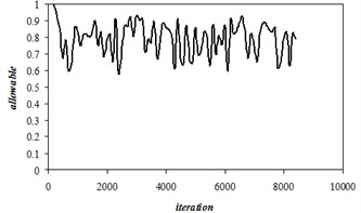
Objective 4 [9] (38 restrictions).

Received for 1200 iterations:

${\mathbf{x}}^{opt}=\left(705.17454;68.6;102.9;282.3249;37.5841\right)$, $F=\mathrm{}$–1.905155. Active restrictions: 1, 2, 34, 37, 38. Fig. 2 shows the proportion of the population of feasible solutions in volume 1000.

Fig. 1Rastrigin function, n=2

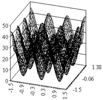
Fig. 2The proportion of feasible solutions

4. Conclusions

The results of solving test problems show that the proposed algorithm can handle all the tasks discussed in [8, 9] for arbitrary restrictions and objective functions. This algorithm is applied to solve further problems for the optimal operation of oil wells.

References

-
Teneev V. A., Shaura A. S., Jakimovich B. A. Structural-Parametric Optimization and Management. Izhevsk State Technical University Publishing House, Izhevsk, 2014, p. 235, (in Russian).
Eshelman L. J., Schaffer J. D. Real-Coded Genetic Algorithms and Interval-Schemata. Foundations of Genetic Algorithms 2. Morgan Kaufman Publishers, San Mateo, 1993, p. 187-202.
Herrera F., Lozano M., Verdegay J. L. Tackling real-coded genetic algorithms: operators and tools for the behavior analysis. Artificial Intelligence Review, Vol. 12, Issue 4, 1998, p. 265-319.
Haupt Randy L., Haupt Sue Ellen Practical Genetic Algorithms. 2nd Edition. John Wiley and Sons, Hoboken, NJ, 2004, p. 261.
Poli Riccardo, Langdon William B., McPhee Nicholas F. A Field Guide to Genetic Programming. Lulu Enterprises, UK, 2008, p. 235.
Tyulenev V. A., Jakimovich B. A. Genetic Algorithms in Modeling Systems. Izhevsk State Technical University Publishing House, Izhevsk, 2010, p. 308, (in Russian).
Prokhorovskaya E. V., Teneev V. A., Shaura A. S. Genetic algorithms with real-coded for solving constrained optimization problems. Intelligent Systems in Production, Vol. 2, 2008, p. 46-55, (in Russian).
Deb K. An efficient constraint handling method for genetic algorithms. Computer Methods in Applied Mechanics and Engineering, Vol. 186, 2000, p. 311-338.
Michalewicz Z. Genetic algorithms, numerical optimization, and constraints. Proceedings of the 6th International Conference on Genetic Algorithms, Morgan Kauffman, San Mateo, 1995, p. 151-158.
About this article