Building surrogate models for two-phase flow of fluids in porous media based on spatial radial basis approximation

1. Introduction and motivation

Consider the simultaneous flow of two distinct phases: wetting and nonwetting fluids. In this case there are four unknown variables and consequently four equations: two differential and two algebraic equations [1]:

where $f=\left\{w,o\right\}$ – subscripts for wetting and nonwetting phases; $S_f$ – saturation, i.e. fraction of the pore volume occupied by phase $f$; $P_c$ – capillary pressure. It is assumed that there is functional relationship between $S_f$ and $P_c$.

The two-phase flow in porous media is nonstationary process even for incompressible flow of fluids in incompressible medium. The simultaneous flow of two fluids causes the phase saturations and relative permeabilities to change over time. Hence, even if flow rates of sources are constant, the reservoir pressure will change over time. To construct approximate solution, we propose a method based on surrogate models. The computational domain is divided into relatively large blocks (coarse grid) that allow us to perform quick calculation using finite-difference method. Spatial refinement (original fine grid) is carried out by radial basis approximation based on calculated parameters of the coarse-grid blocks.

2. The computational model

Let us denote a coarse-grid block by $H=\overline{1,N_B}$, and a fine-grid block of the original grid by $m=\overline{1,M_H}$. The parameters $U=(P_f,S)$ of the corresponding blocks are denoted as $U_m$, $U_H$, $m=\overline{1,M_H}$; $H=\overline{1,N_B}$. The subscript $k\in \left\{i,j\right\}$, $i=\overline{1,n_x}$; $j=\overline{1,n_y}$ corresponds to all blocks of the domain. We will omit the subscript $f$ for the water saturation $S$, because $S_o=1-S_w$. The initial information is numerical solution to Eq. (1) by SS method (simultaneous solution). As was mentioned above it is assumed that there is function $S=F\left(P_c\right)$ and the corresponding inverse function $P_c=F^{-1}\left(S\right)$. Now Eq. (1) can be written in the following form, like in the work [1]:

The coefficients of matrix $D=\left(\begin{array}{ll}{d}_{11}& d_{12}\\ d_{21}& d_{22}\end{array}\right)$ are obtained as a result of linearization of the dependencies $B_f\left(P_f\right)$, $\phi \left(P\right)$, $S\left(P_c\right)$. The coefficients ${\lambda }_f\left(\mathbf{r},S\right)=\mathbf{k}{}_0{}^{\mathrm{}}\mathrm{}\left(\mathbf{r}\right)k_f\left(S\right)/{\mu }_f$ are calculated from relative permeabilities $k_f\left(S\right)$. The empirical formulas of Chang Zhung-Tsang [2] for water and oil phases are used:

The spatial approximation is constructed by using radial functions for steady-state flow of fluids [3, 4]:

To construct radial basis network approximation and to find coefficients ${\alpha }_l$, ${\beta }_l$, $l=\overline{1,L}$ the following steady-state equation is solved:

where${\lambda }_s={\lambda }_w+{\lambda }_o$, ${\gamma }_s={\lambda }_w{\gamma }_w+{\lambda }_o{\gamma }_o/{\lambda }_w+{\lambda }_o$ when $S=\text{0.5}$.

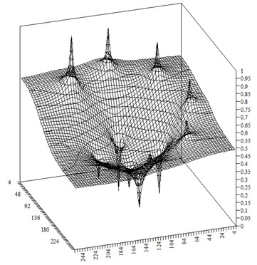
Fig. 1 demonstrates the example of calculation of steady-state pressure field $P_s$.

For each fine-grid blocks contained in the coarse-grid block spatial refinement is achieved through the following approximation:

but this refinement doesn’t involve time and water saturation changes. To account for nonstationary effects Eq. (2) and (1) are solved on coarse grid with blocks $H$ to find $P_f^H\left(t^{n+1}\right)$, $S^H\left(t^{n+1}\right)$ on each time step. To preserve material, balance the following condition should be satisfied:

Let us discretize Eq. (2) for fine grid:

and for coarse grid:

where we denote $\mathrm{\Delta }{P}_f={P_f}^{n+1}-{P_f}^n$, $\mathrm{\Delta }\left(S\frac{\phi }{B_w}\right)={\left(S\frac{\phi }{B_w}\right)}^{n+1}-{\left(S\frac{\phi }{B_w}\right)}^n$.

Fig. 1Distribution of the steady-state pressure field Ps

By summing Eq. (4) for each coarse-grid block and according to Eq. (3) we obtain equations to solve for conversion factors that connect pressure for coarse-grid block and pressure for fine-grid blocks at the given time step:

where ${\omega }_f=\mathrm{\Delta }{P}_f^m/\mathrm{\Delta }{P}_f^H$.

The solution to this system of equations is:

After calculation of the conversion factors for each coarse-grid block, pressure values are updated for the next time steps according to:

Water saturation is calculated from approximate pressure values:

3. Results and discussions

The approximation results are presented with the following example. The domain contains five producers and eight injectors. The injectors are located around the group of the producers.

As it was mentioned, steady-state pressure field $P_s$ is used for training radial basis network and is depicted in Fig. 1. Distribution of the water saturation at time step $\stackrel{-}{t}=\text{1}$ is presented in Fig. 2.

This distribution was obtained by finite-difference method on grid with 256×256 blocks. One can see significant waterflooding of the reservoir compared with initial operating period. The distribution of the approximate water saturation at $\stackrel{-}{t}=\text{1}$ is presented in Fig. 3.

Fig. 2Distribution of the numerical water saturation at time step t-=1

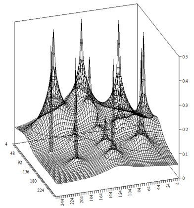
Fig. 3Distribution of the approximate water saturation at time step t-=1

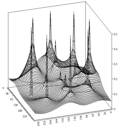
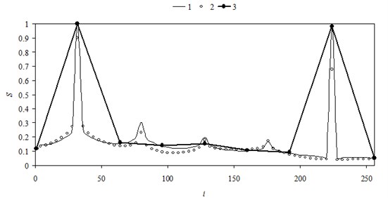
Comparing Fig. 2 and Fig. 3, we see that approximation of the water saturation successfully recognizes spatial features. This is also illustrated in Fig. 4 that shows water saturation changes in midsection of the domain.

The curve 1 corresponds to numerical values obtained by finite-difference method. The curve 2 is approximate values. The curve 3 is obtained by finite-difference method on coarse grid with 16×16 blocks.

Fig. 4Comparison of the water saturation in midsection of the computational domain

4. Conclusions

Suggested method for building the surrogate models of the two-phase flow is based on combination of the finite-difference solution and spatial radial basis approximation. The method allows the use of the approximate models for optimal control the good operation conditions.

References

-
Aziz K., Settari A. Petroleum Reservoir Simulation. Applied Science Publishers, London, p. 1979.
Basniev K. S., Kochina I. N., Maksimov V. M. Underground Hydrodynamics. Nedra, Moscow, 1993, p. 416, (in Russian).
Chanson H. Applied Hydrodynamics: An Introduction to Ideal and Real Fluid Flows. CRC Press, Taylor & Francis Group, Leiden, The Netherlands, 2009, p. 478.
Economides Michael J., Nolte Kenneth G. Reservoir Stimulation. Wiley, USA, 2000, p. 856.
About this article