Abstract
Finite-volume schemes, which honor pressure and flux-continuity conditions, is developed using double quadrature , referred as double family scheme. The scheme is applicable to solve the elliptic pressure equation used in reservoir simulation. Schemes are applicable on both regular cartesian and unstructured triangular meshes. The scheme is defined over a control-volume distributed formulation. The scheme can be applied to both diagonal and full permeability tensor elliptic pressure equation with discontinuous coefficients. The scheme removes the first order errors, which are introduced by standard reservoir simulation schemes when applied to full tensor flow. The scheme is quantified with help of a quadrature rule. When the scheme is applied to highly heterogeneous and anisotropic porous media it does not honor maximum principle resulting in unstable solution with oscillatory behavior. The numerical solution is termed non-monotonicity for high anisotropy ratios with results showing oscillations in the numerical pressure solution. In this paper a double quadrature flux continuous schemes is presented, which with specific choice of quadrature helps in improved stability of the numerical solutions. Numerical convergence of the scheme is also demonstrated with help of a number of numerical test cases and schemes impact on monotonicity behavior is also demonstrated with numerical examples.
Highlights
- Double quadrature
- Gridding
- Numerical Solution
- Numerical Convergence
1. Introduction
Underground porous media reservoirs of hydrogeological flows have complex description in terms of both their physical geometry and geology. Rapid variation in permeability with strong anisotropy is common occurrence in subsurface reservoir simulation, be it for hydrocarbon flows or for underground hydrological studies. Subsurface reservoir simulation requires discretization of continuous flux and pressure equation in order to honor correct local physical interface conditions between the simulation grid blocks, with strong discontinuities and anisotropy in subsurface properties, primarily permeabilities. The derivation of the algebraic flux continuity conditions for full permeability tensor discretization operators has lead to an efficient and robust locally conservative flux-continuous control volume distributed (CVD) finite-volume schemes for determining the discrete pressure and velocity fields in subsurface reservoirs [1-9]. These schemes are also known as multi-point flux approximation or MPFA [10]. Further schemes of this type are presented in [11-13] and more recently in [14, 15]. These numerical schemes could be applied to the diagonal and full tensor elliptic pressure equation with rapid variations in permeability and remove the first order error in numerical approximation in typical reservoir simulation results, which are often based on two-point flux approximation, when applied to full tensor flow approximation. Some other numerical schemes of similar types that also preserve continuity of fluxes have also been developed using mixed finite element methods [16-18] and discontinuous galerkin finite element methods [19, 20]. Numerical convergence of these numerical scheme on unstructured and structured meshes has also been presented earlier in a number of papers [9, 21-23].
When these numerical schemes are applied to strongly anisotropic heterogeneous porous media they fail to satisfy a maximum principle (similar to finite eminent, mixed finite element and other finite-volume methods) and result in loss of solution stability, particularly, for very high anisotropy ratios, which often lead to spurious oscillations in the numerical pressure solution. Some work has been carried out previously with aim of preserving stability of the numerical solutions for highly heterogeneous cases with skewed meshes, please see references [3, 6, 24].
Monotonicity conditions were first derived in [1] for an M-matrix and later in [25] for a monotone matrix. Numerical treatment based on mesh/grid optimization methods have been used to help improve stability of the discrete system [26]. Still, all of the published numerical schemes show only a limited impact and their stability is often subject to the order of magnitude of the permeability anisotropy ratios. A more promising strategy based on Flux-splitting techniques has been presented in [7, 8, 27], which helps in locally imposing maximum principle and resulting numerical solutions are oscillation free. Therefore, guaranteeing a more stable numerical pressure solution.
Conditions for the (one parameter) family of flux-continuous schemes to possess symmetric positive definite matrices and for such schemes to have M-matrices with diagonal dominance and negative off-diagonals are presented in [1, 2]. The discretized system obtained for the schemes in the case of a full tensor are shown to be conditionally diagonally dominant and thus the M-matrix property is conditional [1, 28]. For very large anisotropic ratios with skewed meshes, the resulting numerical system for these schemes can be unstable (as in the case of other numerical techniques like FEM & FVM) and the numerical pressure solutions can consequently exhibit oscillatory behavior. This paper is focused on seeking the most robust numerical approximation with help of double parameter scheme. Numerical convergence of the double parameter schemes is demonstrated with help of series of numerical test cases.
This paper is organized as follows: Description of the single phase flow problem encountered in reservoir simulation with respect to the general tensor pressure equation is given in Section 2. Details of the numerical construction of the double parameter scheme with discretization in physical space are presented in Section 3. Section 4 details the precise conditions required to obtain a stable numerical solution and shows the performance of the scheme with respect to stability conditions. Section 5 presents the numerical convergence results with help of a series of test cases. Section 6 presents numerical examples that demonstrate the impact of scheme quadrature choice on monotonicity behavior with help of some numerical examples. Finally, conclusions are presented in Section 7.
2. Problem description and governing equations
The typical formulation of Darcy’s law states that the problem is to find the pressure satisfying:
over a given domain , subjected to a given (Neumann/Dirichlet) boundary conditions on a given boundary . The right hand side term represents a flow rate and . The permeability Matrix can either be a diagonal or full cartesian tensor, which has the general form:
The resulting pressure equation with full permeability matrix is assumed to be elliptic such that:
The permeability tensor can be discontinuous across internal boundaries of the domain . The boundary conditions, which are imposed here are of Dirichlet and Neumann type. For incompressible fluid flow in porous media – pressure need to be specified at at-least at one point in the domain to obtain a numerical solutions. For subsurface reservoir simulation, Neumann boundary conditions on requires no-flux on the domain boundary such that , where is the outward normal vector to .
2.1. Elliptic pressure equation
The pressure equation presented in the section above is given in the physical space w.r.t the classical Cartesian coordinate system. In this section we present the elliptic pressure equation in a general curvilinear coordinate system that is defined with respect to a uniform dimensionless transform space with a coordinate system. Choosing domain to represent a control volume comprised of surfaces that are tangential to constant respectively, Eq. (1) is integrated over via the Gauss divergence theorem to yield:
where is the boundary of and is the unit outward normal. Spatial derivatives are computed using:
where is the Jacobian. Resolving the , components of velocity along the unit normals to the curvilinear coordinates , e.g., for constant, gives rise to the general tensor flux components:
where general tensor has elements defined by:
and the closed integral can be written as:
where e.g. is the difference in net flux with respect to and , . This condition demonstrates that any such scheme applicable to a full matrix permeability tensor could also be applied to non-K-Orthogonal grids. Note that , and ellipticity of follows from Eqs. (3 and 7). Full permeability tensors can arise from upscaling, and local orientation of the grid and the permeability field. For example, by Eq. (7), a diagonal anisotropic Cartesian tensor leads to a full tensor on a curvilinear orthogonal grid [23] (a grid is called orthogonal if all grid lines intersect at a right angle).
3. Flux-continuous finite volume schemes
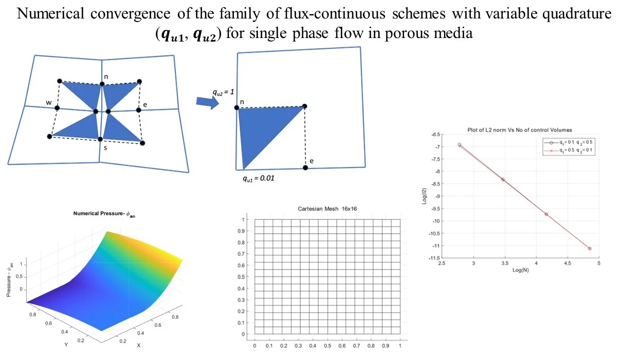
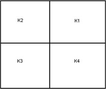
Finite volume schemes, which honor local pressure and flux continuity conditions and are locally conservative have been presented in [1-6]. The schemes have been developed for different grid types structured and unstructured grids in physical space and transform space. Numerical convergence for a range of quadrature in physical and transform space have been presented in [5]. The schemes have continuity of pressure and flux across primal grid cell control-volume interfaces (Control Volume is defined as the volume over which mass can transfer in and out across its boundary (Pal 2006)). Here we present a short summary of the structured cell centred quadrilateral formulation. The nine point support of the numerical scheme is shown in Fig. 1(a)). The numerical scheme has flow and rock variables (porosity, permeability etc.) defined at the cell centre, with this definition, the discrete approximation points are at then located at the centres of the primal grid cells, which are also the control-volumes. For each group of four nodes, four triangles are drawn as in Fig. 1(a). Each group of nodes are defined within a dual-cell (each group of four cell-centered nodes surrounding a primal grid vertex defines the fundamental corners of a dual cell) which is obtained by joining cell centres with cell edge mid-points as indicated by the dashed contour in Fig. 1(b). The dual cells partition the primal cells (or control-volumes) into subcells (the dual cells partition the primal quadrilateral grid cells (or control volumes) into sub-quadrilateral cells, which are called subcells). Two faces of each subcell also define sub faces of two faces of the parent control-volume.
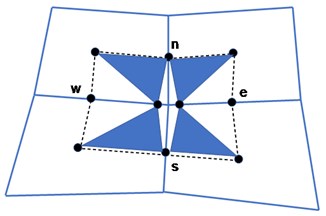
Fig. 1a) Flux-continuity at specific north, south, east and west location n,s,e,w on the control-volume sub-cell faces, b) location of quadrature points (qu1,qu2) on the sub-cell face
a)
b)
3.1. quadrature schemes
Flux continuous schemes are formulated using the principle of pressure and flux continuity conditions on the control-volume subcell faces. The continuity conditions are shown conceptually with help of the Fig. 1(a). It can be seen in the figure that the continuity conditions is met at the four positions , corresponding to north, south, east and west faces. The area is shown with help of shaded triangles and their point of contact in the Fig. 1(b). On each control-volume cell sub-face the point of continuity is parameterized with help of the variable quadrature depending on the location of continuity at the sub-face, please see Fig. 1(b) . For any given control-volume subcell, the points of continuity of flux and pressure could be located anywhere in the ranges on the two faces of each subcell. The precise values of define the quadrature points, thereby, resulting in the formulation corresponding to families schemes, which are flux-continuous. Fig. 1(b) shows a conceptual plot for quadrature points located at and . Cell face pressures , , , are introduced at , , , locations. Pressure sub-triangles are defined with local triangular support imposed within each quarter (sub-cell) of the dual-cell as shown in Fig. 1(b). Pressure , in local cell coordinates, is piecewise linear over each triangle. The physical space flux-continuity conditions for cells 1 to 4, sharing a common grid vertex inside the dual-cell are expressed as:
The parametric variation in is illustrated further using the sub-cell example of Fig. 1(c), with sub-cell containing sub-triangle . Let denote the coordinates of the cell-centre and , denote the local continuity coordinates. Then it is understood that the continuity position is a function of with and .
Piecewise constant fluxes are then computed on every pressure sub-triangles belonging to the sub-cells of the dual-cell as shown in Fig. 1(b). The local linear pressure , is expanded in sub-triangle coordinates. The Darcy flux approximation for sub-triangle is given below:
and:
Using Eqs. (10, 11) the discrete Darcy velocity is defined as:
where is the local permeability tensor of cell 1 and dependency of on quadrature point arises through:
where approximate and are defined by Eq. (11). The normal flux at the left hand side of (Fig. 1(b)) is resolved along the outward normal vector (Fig. 1(b) and is defined in terms of the general tensor as:
and the resulting coefficients of denoted by and are sub-cell (physical-space) approximations of the general tensor components (Eq. (9)) at the left hand face at S, and are functions of . A similar expression for flux is obtained at the right hand side of S from cell 2 (Fig. 1(b). Similarly sub-cell fluxes are resolved on the two sides of the other faces at W, N and E. Flux continuity is then imposed across the four cell interfaces at the four positions N, S, E and W (Fig. 1(a) which are specified according to quadrature point . The local physical space flux continuity conditions are now defined in the dual cell and expressed as follows.
The above system of Eq. (9) is now expressed as:
where are the fluxes defined in the dual-cell and are the interface pressures. Similarly are the cell centered pressures. Thus the four interface pressures are expressed in terms of the four cell centered pressures. Using Eq. (15), is now expressed in terms of to obtain the dual-cell flux and coefficient matrix:
Thus, the cell-face pressures are eliminated from the flux by being determined locally in terms of the cell centered pressures in a preprocessing step, avoiding introduction of the interface pressure equations into the assembled discretization matrix. The Eq. (16) can also be written as:
where the entries of matrix are accumulated inverse tensor elements and are the differences of vertex pressures. Consistency of the formulation follows from Eq. (17) which shows that flux is zero for constant potential. The relationship with the mixed method can also be deduced from Eq. (17), [2] from which it also follows that the above systems Eqs. (16), (17) represent the generalisation of the standard flux with harmonic coefficients to general elements with families of schemes defined by quadrature point , see [2, 4, 9, 21-23] for details. The physical space formulation does not posses a symmetric discretization matrix for arbitrary quadrilaterals, however, transform space (cell and sub-cell) formulations that are symmetric positive definite are presented in [1, 4]. Flux continuity in the case of a general-tensor is obtained while maintaining the standard single degree of freedom per cell. Since the continuity equations depend on both and (unless a diagonal tensor is assumed with cell-face midpoint quadrature resulting in a 2-point flux), the interface pressures are locally coupled and each group of four interface pressures is determined simultaneously in terms of the group of four cell centered pressures whose union contains the continuity positions. Finally for a structured grid the scheme is defined by:
where , are the integer coordinates of the central quadrilateral cell, Fig. 1(a)) and:
where , denote the “integer” coordinates of the top right hand side dual-cell, Fig. 1(a)). The unstructured formulation is presented in [22, 23].
4. Monotonicity
Flux-continuous schemes results in a discrete matrix which has five to nine diagonals in two dimensions and three to twenty-seven diagonals in three dimensions on a structured mesh. The discrete matrix can be expressed as:
where is the matrix of discrete operator, is the unknown pressure and is the source term. Ideally the discrete system obtained in this way should results in an Eq. (20), which should be a nonsingular matrix and should satisfy maximum principle that is comparable to the continuous counterpart of the discrete problem. The condition ensures that the numerical solution obtained in this way is free from any non-physical oscillations. The maximum principle is satisfied for the discrete system given in 20 if the discrete matrix operator is a monotone. The matrix operator, of the discrete system, is a non-singular monotone matrix if it obeys the following condition [29]:
where is a null matrix. A sufficient condition for a maximum principle that can ensure that non-physical oscillations do not occur in the resulting discrete solution is that is an M-matrix, i.e. monotone or positive definite with , .
4.1. M-matrix conditions
The following set of conditions are often easier to verify.
is an M-matrix if:
In addition, must be either strictly diagonally dominant (strict inequality in the latter of Eq. (22) or weakly diagonally dominant with strict inequality for at least one row, must also be irreducible. The first M-matrix analysis for schemes of this type is presented in [1], where conditions for nine-node flux continuous schemes to be an M-Matrix are:
and is a function of quadrature point. One of the essential conditions here is that:
which is only sufficient for ellipticity [1] and therefore quite limiting on the range of tensors that are applicable. Tensors that are elliptic with:
and are such that violate the M-Matrix criteria of Eq. (23) and expose the M-Matrix limit.
5. Numerical results: numerical convergence study
While numerical convergence tests for transform and physical space formulations on cartesian and triangular unstructured meshes in two-and three dimensions have previously been performed by [5, 21-23] for the default member of the family of flux-continuous MPFA schemes i.e. for 1.
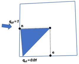
The aim of the numerical convergence study presented here is to test the effect of variable quadrature points , on the numerical convergence of the scheme. Although a number of quadrature combinations exist for , , only two specific combination of quadrature points are evaluated 0.5, 0.1 and 0.1, 0.5.
In this section numerical convergence results are presented cartesian grids in two dimensions. In all test cases the permeability field remains unchanged under grid refinement, ensuring that each problem is invariant with respect to each grid level for the convergence study. The classical norm is used to measure errors in fluxes and pressure, which is defined for fluxes and pressure as:
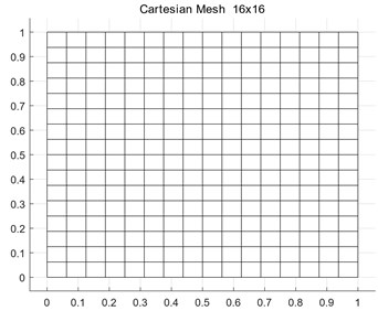
where, (where ) is the edge normal flow velocity. Subscript refers to numerical solution. Further is the volume of the grid cell , and is the volume associated with edge (where two cells are separated by edge ). The grid refinement levels used for the norm calculation where mesh sizes of 16×16, 32×32, 64×64, and 128×128 are used for all test cases in 2D. In each case Dirichlet boundary conditions are prescribed via the exact solutions.
5.1. Numerical test 1: uniformly discontinuous permeability
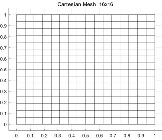
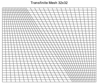
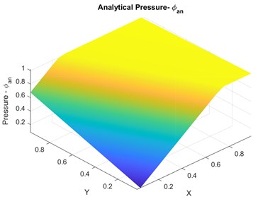
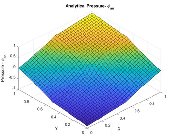
In this case the pressure field is piecewise quadratically varying over the domain shown in Fig. 2(a). Fig. 2(b) shows analytical pressure results on this test case. Fig. 2(c) shows typical mesh used for the numerical convergence in this case. The domain is discontinuous with discontinuity aligned along the line , and the analytical solution is given as:
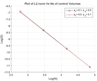
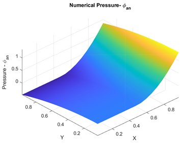
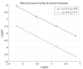
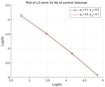
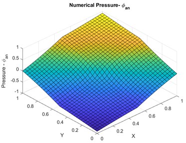
The imposed top boundary flux is also discontinuous at , resulting in a discontinuous tangential flux across the domain. The computed numerical solution and the plots showing norm of pressure for the varying quadrature and are shown in Fig. 3(a) and (b), respectively. accuracy is observed in numerical pressure solution for and and accuracy is observed in numerical pressure solution for and .
Fig. 2Case 1: a) Discontinuity of the domain under consideration, b) exact analytical solution for pressure, c) sample mesh used for numerical convergence
a)

b)
c)
Fig. 3Case 1: a) convergence plots for qu1, qu2. b) exact numerical pressure – physical space
a)
b)
5.2. Numerical test 2: non-uniform discontinuous permeability field
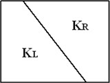
In this case the medium is divided into two parts as, see Fig. 4(a). The permeability is discontinuous and permeability ratio is 1/10 across the medium discontinuity. The discontinuity is aligned along the line , where and .The pressure is piecewise linear and varies as:
The diagonal permeability tensor , where for and for . The numerical solution shown in Fig. 4(b) was obtained using a grid aligned along the discontinuity. Typical mesh used for the numerical convergence is shown in Fig. 4(c). Numerical convergence for varying and quadrature is shown in Fig. 5(a) and the numerical pressure Physical space for the varying quadrature is shown in Fig. 5(b). accuracy is observed in numerical pressure solution for and and accuracy is observed in numerical pressure solution for and .
Fig. 4Case 1: a) discontinuity of the domain under consideration, b) exact analytical solution for pressure, c) sample mesh used for numerical convergence
a)

b)
c)
Fig. 5Case 1: a) convergence plots for qu1, qu2, b) Exact numerical pressure – physical space
a)
b)
5.3. Numerical test 3: permeability field with internal discontinuity
This case involves an internal discontinuity. The problem involves a rectangular domain with internal discontinuous permeability variation as indicated in Fig. 6(a). The exact solution in each case takes the form:
The exact analytical pressure solution is shown in Fig. 6(b) and the cartesian mesh used in this case is shown in Fig. 6(c). Numerical convergence for varying and quadrature is shown in Fig. 7(a) and the numerical pressure Physical space for the varying quadrature is shown in Fig.7(b). accuracy is observed in numerical pressure solution for and and accuracy is observed in numerical pressure solution for and .
Fig. 6a) Internal discontinuity along θ=π/2, b) exact analytical pressure, c) sample mesh used for numerical convergence
a)
b)
c)
Fig. 7Case 1: a) convergence plots for q1, q2, b) exact numerical pressure – physical space
a)
b)
6. Numerical results: test of monotonicity behavior
In this section a series of numerical test are presented to test the quasi-monotonic property of the variable quadrature points scheme. The test examples involve subsurface permeability discontinuity with highly heterogeneous and anisotropic permeability tensor.
6.1. Test case 1: v shape permeability distribution
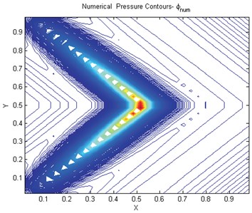
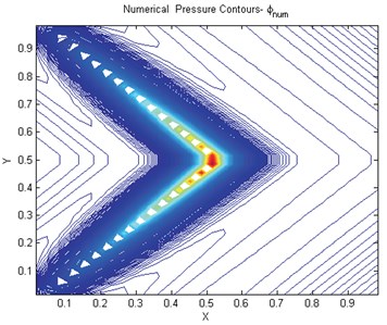
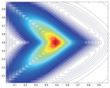
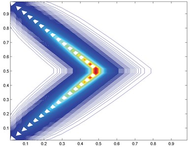
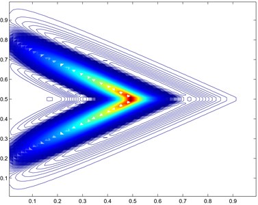
In this test case, a two dimensional domain with a permeability tensor that changes direction in anisotropy halfway across the domain going from = [1, 0.99, 0.99, 1] to = [1, –0.99, –0.99, 1], as shown in Fig. 8, is investigated. A point source is placed in the centre of the 2D domain (of unit length in and direction) and Dirichlet conditions are applied. In this test case due to discontinuity in permeability tensor M-matrix conditions are tested under variable coefficient conditions. Fig. 9(a) shows the results with with visible spurious oscillations. In the second case using the different choice of quadrature parameter with 0.01 oscillation free results are obtained, see Fig. 9(b).
Fig. 8Change in direction of anisotropy in Permeability Tensor at y=0.5
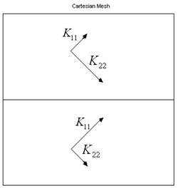
Fig. 9a) Numerical pressure contours with instabilities like oscillations qu1=qu2=q=1, b) numerical pressure contours free of instabilities e.g., no oscillation. qu1=qu2=q=0.01
a)
b)
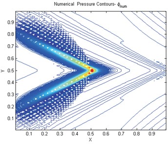
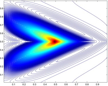
Results using the double family with 0.005025125, are shown in Fig. 10. In these cases the M-matrix conditions are satisfied. Using a reduced support scheme (7-point – constant tensor) motivated by the above analysis yields the result in Fig. 11(a). If the alternative orientation is selected the scheme still has reduced support and the scheme does not posses an M-matrix and the result obtained is shown in Fig. 11(b). There are clear oscillations and spread in the solution in this case, which serves as a test of the angled condition.
6.2. Test case 2: strong anisotropic permeability distribution
In this case the same boundary conditions apply as in case 2. The permeability tensor changes direction in anisotropy halfway across the domain as before, now with stronger tensor field, going from [750.25 432.58 432.58 250.75] to [750.25 –432.58 –432.58 250.75] as indicated in Fig. 8. In this case the tensor has a principal anisotropy ratio of 1/1000, while the tensor is elliptic, the sufficient condition for ellipticity, is clearly violated. Consequently, the conditions for an M-matrix are also violated.
Fig. 10Numerical pressure contours free of instabilities like oscillations for double quadrature qu1= 0.005025125, qu2= 1
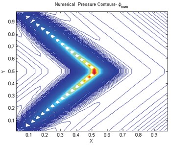
Fig. 11a) Numerical pressure 7-pt scheme tensor not aligned with scheme stencil, b) numerical pressure contours 7-pt scheme tensor aligned with scheme stencil
a)
b)
Fig. 12a) Numerical pressure contours 9-pt scheme tough tensor, q=1
Results are presented for and Fig. 12 for a 64×64 grid. There are strong oscillations in the solution showing clear violation of the maximum principle. Next, we turn to the reduced support scheme with angled approximation with orientation of opposite sign to the cross terms, results are in Fig. 13(a) which show severe oscillations. Finally, we employ the reduced support scheme with angled approximation and orientation that matches the sign of the cross terms, consistent with the M-matrix analysis, for the same 64×64 grid Fig. 13(b). While oscillations are present, they are seen to be reduced. The results clearly show a reduction in oscillations in each case, however at each grid level and as convergence is approached, the consistent reduced support scheme yields almost oscillation free results or quasi-monotonic.
Fig. 13a) Numerical pressure contours 7-pt scheme tough tensor not aligned with scheme stencil, b) numerical pressure 7-pt scheme tough tensor aligned with scheme stencil
a)
b)
7. Conclusions
A two parameter scheme is presented, which is locally conservative and grantees continuity of flux and pressure. Numerical convergence of the scheme is also presented, which shows numerical accuracy of order on the tested examples.
When a classical scheme is used that violates the governing conditions oscillations appear in the solutions. In this paper results are presented for highly anisotropic full-tensor fields that verify that double family scheme offers quasi-monotonic behavior. When the governing conditions are satisfied the for given choice of quadrature the numerical pressure solution is free oscillations.
The variable support schemes are able to compute numerical pressure solutions with minimal or no oscillations and has much improved resolution compared to schemes relying on fixed quadrature rules. The scheme also proves effective for high anisotropy ratios.
References
-
M. G. Edwards and C. F. Rogers, “Finite volume discretization with imposed flux continuity for the general tensor pressure equation,” Computational Geosciences, Vol. 2, No. 4, pp. 259–290, 1998, https://doi.org/10.1023/a:1011510505406
-
M. G. Edwards, “Unstructured, control-volume distributed, full-tensor finite-volume schemes with flow based grids,” Computational Geosciences, Vol. 6, No. 3/4, pp. 433–452, 2002, https://doi.org/10.1023/a:1021243231313
-
M. G. Edwards, “M-Matrix flux splitting for general full tensor discretization operators on structured and unstructured grids,” Journal of Computational Physics, Vol. 160, No. 1, pp. 1–28, May 2000, https://doi.org/10.1006/jcph.2000.6418
-
M. G. Edwards and M. Pal, “Symmetric positive definite general tensor discretization: a family of sub-cell flux continuous schemes on cell centred quadrilateral grids,” (in press).
-
M. Pal, M. G. Edwards, and A. R. Lamb, “Convergence study of a family of flux‐continuous, finite‐volume schemes for the general tensor pressure equation,” (in Press), International Journal for Numerical Methods in Fluids, Vol. 51, No. 9-10, pp. 1177–1203, Jul. 2006, https://doi.org/10.1002/fld.1211
-
Mayur Pal and Michael G. Edwards, “Effective upscaling using a family of flux-continuous finite-volume schemes for the pressure equation,” in ACME UK, Apr. 2006.
-
M. Pal and M. G. Edwards, “Family of flux-continuous finite-volume schemes with improved monotonicity,” in Proceedings of the 10th European Conference on the Mathematics of Oil Recovery, 2006.
-
M. Pal and M. G. Edwards, “Flux-Splitting Schemes for improved montonicity of discrete solution of elliptic equation with highly anisotropic coefficients,” in ECCOMAS CFD 2006: Proceedings of the European Conference on Computational Fluid Dynamics, 2006.
-
M. Pal and M. G. Edwards, “Non‐linear flux‐splitting schemes with imposed discrete maximum principle for elliptic equations with highly anisotropic coefficients,” International Journal for Numerical Methods in Fluids, Vol. 66, No. 3, pp. 299–323, May 2011, https://doi.org/10.1002/fld.2258
-
I. Aavatsmark, “Introduction to multipoint flux approximation for quadrilateral grids,” Computational Geosciences, Vol. 6, No. 3/4, pp. 405–432, 2002, https://doi.org/10.1023/a:1021291114475
-
S. H. Lee, P. Jenny, and H. A. Tchelepi, “A finite-volume method with hexahedral multiblock grids for modeling flow in porous media,” Computational Geosciences, Vol. 6, No. 3/4, pp. 353–379, 2002, https://doi.org/10.1023/a:1021287013566
-
S. Verma, “Flexible grids for reservoir simulation,” Ph.D. Thesis, Stanford University, 1996.
-
S. K. Khattri, “Analyzing finite-volume for single-phase flow in porous media,” Journal of Porous Media, Vol. 10, No. 2, pp. 109–123, 2007.
-
O. Iliev and I. Rybak, On Approximation Property of Multipoint Flux Approximation Method. 2007.
-
A. A. Lukyanov, “A meshless multi-point flux approximation method,” in Numerical Analysis and Applied Mathematics ICNAAM 2012: International Conference of Numerical Analysis and Applied Mathematics, 2012, https://doi.org/10.1063/1.4756377
-
L. J. Durlofsky, “A Triangle Based Mixed Finite Element-Finite Volume Technique for Modeling Two Phase Flow through Porous Media,” Journal of Computational Physics, Vol. 105, No. 2, pp. 252–266, Apr. 1993, https://doi.org/10.1006/jcph.1993.1072
-
A. S. Abushaikha, D. V. Voskov, and H. A. Tchelepi, “Fully implicit mixed-hybrid finite-element discretization for general purpose subsurface reservoir simulation,” Journal of Computational Physics, Vol. 346, pp. 514–538, Oct. 2017, https://doi.org/10.1016/j.jcp.2017.06.034
-
A. S. Abushaikha and K. M. Terekhov, “A fully implicit mimetic finite difference scheme for general purpose subsurface reservoir simulation with full tensor permeability,” Journal of Computational Physics, Vol. 406, p. 109194, Apr. 2020, https://doi.org/10.1016/j.jcp.2019.109194
-
B. Rivière, M. F. Wheeler, and K. Banaś, “Discontinuous Glaerkin method applied to a single phase flow in porous media,” Computational Geosciences, Vol. 4, No. 4, pp. 337–349, 2000, https://doi.org/10.1023/a:1011546411957
-
T. F. Russell and M. Wheeler, “Mathematics of reservoir simulation: finite element and finite difference methods for continuous flows in porous media,” in Frontiers in Applied Mathematics SIAM, 1983, p. 35.
-
M. Pal and M. G. Edwards, “The competing effects of discretization and upscaling – a study using the q-family of CVD-MPFA,” 11th European Conference on the Mathematics of Oil Recovery, Vol. 68, No. 1, Sep. 2008, https://doi.org/10.3997/2214-4609.20146372
-
M. Pal and M. G. Edwards, “A family of multi-point flux approximation schemes for general element types in two and three dimensions with convergence performance,” International Journal for Numerical Methods in Fluids, Vol. 69, No. 11, pp. 1797–1817, Aug. 2012, https://doi.org/10.1002/fld.2665
-
Mayur Pal, “Families of control-volume distributed CVD(MPFA) finite volume schemes for the porous medium pressure equation on structured and unstructured grids,” Ph.D. thesis, Swansea University, 2007.
-
J. M. Nordbotten and G. T. Eigestad, “Discretization on quadrilateral grids with improved monotonicity properties,” Journal of Computational Physics, Vol. 203, No. 2, pp. 744–760, Mar. 2005, https://doi.org/10.1016/j.jcp.2004.10.002
-
J. Nordbotten and I. Aavatsmark, “Monotonicity conditions for control volume methods on uniform parallelogram grids in homogeneous media,” Computational Geosciences, Vol. 9, pp. 61–72, 2005.
-
M. J. Mlacnik and L. J. Durlofsky, “Unstructured grid optimization for improved monotonicity of discrete solutions of elliptic equations with highly anisotropic coefficients,” Journal of Computational Physics, Vol. 216, No. 1, pp. 337–361, Jul. 2006, https://doi.org/10.1016/j.jcp.2005.12.007
-
T. Aadland, I. Aavatsmark, and H. K. Dahle, “Performance of a flux splitting scheme when solving the single-phase pressure equation discretized by MPFA,” Computational Geosciences, Vol. 8, No. 4, pp. 325–340, Dec. 2004, https://doi.org/10.1007/s10596-004-3774-y
-
G. T. Eigestad, I. Aavatsmark, and M. Espedal, “Symmetry and M-Matrix issues for the O-Method on an unstructured grid,” Computational Geosciences, Vol. 6, No. 3/4, pp. 381–404, 2002, https://doi.org/10.1023/a:1021239130404
-
O. Axelsson, Iterative Solution Methods. Cambridge University Press, 1994, https://doi.org/10.1017/cbo9780511624100
-
I. Aavatsmark, G. T. Eigestad, B. T. Mallison, and J. M. Nordbotten, “A compact multipoint flux approximation method with improved robustness,” Numerical Methods for Partial Differential Equations, Vol. 24, No. 5, pp. 1329–1360, Sep. 2008, https://doi.org/10.1002/num.20320
About this article

