On the inversion of describing functions in nonlinear system analysis

Du, Huan; Li, Zhiqiang; Ahlin, Kjell

doi:10.21595/vp.2017.18538

Vibroengineering Procedia

Browse Procedia

Published: 30 June 2017

Check for updates

On the inversion of describing functions in nonlinear system analysis

Huan Du¹

Zhiqiang Li²

Kjell Ahlin³

^{1, 2}School of Reliability and System Engineering, Beihang University, Beijing, China

³Xielalin Consulting, Akersberga, Sweden

Corresponding Author:

Zhiqiang Li

Cite the article Download PDF

Downloads 1806

CrossRef Citations 2

Abstract

Nonlinear mechanical vibrations are widely found in engineering structures. Traditional linear analysis methods are failing to meet the growing requirements of analysis accuracy. Because of the complexity of nonlinear system, there is no general method for nonlinear system analysis. Based on the describing function method, a polynomial inversion method may be used in nonlinear system identification. Using this method, the measured DF can be inverted into the form of force which has a clearer physical meaning and is easier to use for parameter fit. A MDOF system with two types of nonlinearities at the same location is studied to demonstrate this method.

1. Introduction

In the past, most attention was paid to linear systems, and theories and methods have been developed for linear system modeling, simulation and prediction. However, there exist lots of nonlinearities in an actual engineering system and some of them may have a significant effect in system dynamic characteristics. The study of nonlinearities is indispensable and inevitable. However, one should be forced to admit that there are no general analysis methods that can be applied to all nonlinear system in all instances [1].

During the past decades, lots of work has been done in identification of system nonlinearities and they can be roughly divided into two categories, time domain methods and frequency domain methods. Time domain identification of nonlinear structural models relies on processing time series while the data processing in frequency domain methods can take form of Fourier spectra, frequency response and transmissibility functions, or power spectral densities [2]. The describing function, DF, based on the definitions of the frequency response function and the first-order harmonic balance method, was used in analyzing nonlinear structures by Tanrikulu O., et al. [3]. A further research was made by Özer and Özgüven [4] in calculating the describing function’s approximate solutions by using the Sherman-Morrison Method. Aykan and et al [5] proposed a method to transform the describing function into the restoring force to make it more visualized.

Finding the nonlinear forces corresponding to the measured describing functions is called describing function inversion [6]. In this paper, nonlinear system identification using describing function is introduced briefly. A polynomial inversion method of inverting the measured describing function is proposed. At last, an illustrative example is given to demonstrate this method.

2. Theory

2.1. Describing function method

The use of non-linear describing function matrix to represent the nonlinear forces in a MDOF system was proposed and developed by Özer et al. [4]. They established a set of feasible methods for nonlinear system identification, including early detection, nonlinear localization and parameter estimation. This method was confirmed to have an acceptable application to a MDOF system with several nonlinearities at different locations in a case study [7]. As this method was discussed in detail in ref. [7], a brief introduction is given below for readers’ comprehension.

The equation of motion for a nonlinear MDOF system under excitation can be written as:

1

[M] ∙ \{\ddot{x}\} + [C] ∙ \{\dot{x}\} + [K] ∙ \{x\} + \{n l f (x, \dot{x})\} = \{f\},

where $[M]$ , $[C]$ , and $[K]$ are mass, viscous damping and stiffness matrices of the linear system, respectively. $\{f\}$ and $\{x\}$ stand for the external forces and the responses of the system. $\{n l f (x, \dot{x})\}$ represents the nonlinear internal forces in the system, and it is a function of the displacement and/or velocity responses, depending on the type of nonlinearity present in the system.

A harmonic excitation with circular frequency $ω$ may be written:

2

\{f\} = \{F\} e^{j ω t} .

Using first order harmonic balance method, the response is assumed to consist of only the first fundamental harmonic, disregarding higher order harmonics. Since the response is harmonic as the assume, $\{x\} = \{X\} e^{j ω t}$ , the internal nonlinear forces can be harmonic too:

3

\{n l f (x, \dot{x})\} = [∆ (x, \dot{x})] \{X\} e^{j ω t},

where $[∆ (x, \dot{x})]$ is the ‘non-linearity matrix’ that is dependent on response amplitude. The “non-linearity matrix” can be formed by using describing function $v$ representations of internal non-linear forces as follows:

4

∆_{r r} = v_{r r} + \sum_{j = 1, j \neq r}^{n} v_{r j},

5

∆_{r j} = {- v}_{r j} .

The relationship between describing functions and nonlinear forces will be introduced in Section 2.2. From the equations above:

6

(- ω^{2} ∙ [M] + j ∙ ω ∙ [C] + [K]) ∙ \{X\} + [∆] ∙ \{X\} = \{F\} .

Then the nonlinear frequency response function (FRF) matrix $[H^{N}]$ can be calculated as:

7

[H^{N}] = {(- ω^{2} ∙ [M] + j ∙ ω ∙ [C] + [K] + [∆])}^{- 1} .

The FRF of underlying linear system, $[H^{L}]$ , can be written as:

8

[H^{L}] = {(- ω^{2} ∙ [M] + j ∙ ω ∙ [C] + [K])}^{- 1} .

Notice that the nonlinear FRF may be different at different excitation levels due to the non-linearity matrix. The non-linearity matrix can formally be obtained by:

9

[∆] = {[H^{N}]}^{- 1} - {[H^{L}]}^{- 1} .

Eq. (9) is the core of this method. Once we get the non-linearity matrix, we have the ability to localize and identify the nonlinearities in a MODF system. Although there still exist some challenges, such as the calculation of $[H^{L}]$ and $[H^{N}]$ , they were discussed and partially solved in previous studies mentioned above. Readers who are interested can have a more comprehensive understanding in ref. [4, 7].

2.2. Polynomial inversion method

By the use of DF method, the nonlinear force describing function of the response’s amplitude can be obtained. Generally, they are represented in the form of two related series, the response amplitude, $\{d f x\}$ , and corresponding DF values, $\{d f\}$ . The describing function, which can be used for determining the type of nonlinearity as well as for parametric identification, has a quite complex form and it will be worse if there exist multiple nonlinearities in one location of the nonlinear system. This not only makes it necessary for a wealth of engineering experience but also greatly increases the difficulty for identification. An inversion method that works for general describing functions will effectively solve this problem. In the rest of this section, a polynomial inversion method will be given in detail.

The describing function for general dynamic system nonlinearity can be written as:

10

v (x, \dot{x}) = \frac{j}{π A} \int_{0}^{2 π} n l f (x, \dot{x}) e^{- j τ} d τ,

where the response $x$ is supposed to be:

11

x (t) = A s i n (ω t + θ) = A s i n (τ),

12

τ = ω t + θ .

Eq. (10) indicates that the describing function is a complex function, and a complex function can be divided into two parts, real part and imaginary part:

13

v (x, \dot{x}) = v_{p} (x, \dot{x}) + j {∙ v}_{q} (x, \dot{x}) .

The real part $v_{p}$ corresponds to stiffness nonlinearities while the imaginary part $j {∙ v}_{q}$ corresponds to damping nonlinearities [8]. For each part, the derivation for the inverse is given as follows:

An arbitrary nonlinearity can be expressed as a sum of n nonlinearities, $N_{1}$ , $N_{2}$ ,..., $N_{n}$ :

14

n l f (x) = {n l f}_{1} (x) + {n l f}_{2} (x) + \dots + {n l f}_{n} (x) = \sum_{i = 1}^{n} {n l f}_{i} (x) .

The DF for composite nonlinearities is given by:

15

v (A) = \frac{j}{π A} \int_{0}^{2 π} \sum_{i = 1}^{n} {n l f}_{i} (A s i n τ) e^{- j τ} d τ = \frac{j}{π A} \sum_{i = 1}^{n} \int_{0}^{2 π} {n l f}_{i} (A s i n τ) e^{- j τ} d τ = \sum_{i = 1}^{n} v_{i} (A) .

Eq. (14) and Eq. (15) indicate that the DF and the inverse DF transformations satisfy the superposition principle. By polynomial fitting, an arbitrary function can be approximately represented in the form of a sum of polynomials. Theoretically, the higher the polynomial order we use, the more accurate result we will get.

Because the DF yields zero when the corresponding force is even, we represent the input-output characteristic for a nonlinearity as an odd nth-order polynomial:

16

n l f (x) \approx c_{1} x {+ c}_{2} x |x| + \dots + c_{n - 1} x^{n - 2} |x| + c_{n} x^{n} .

The $m$ th item of DF can be computed by integrating over the interval $0 < τ < π / 2$ , as:

17

v_{m} (A) = \frac{4}{π A} \int_{0}^{\frac{π}{2}} {n l f}_{m} (A s i n τ) s i n τ d τ = \frac{4}{π A} \int_{0}^{\frac{π}{2}} c_{m} {(A s i n τ)}^{m} s i n τ d τ

= \{\begin{matrix} c_{m} \frac{m (m - 2) (m - 4) \dots (3)}{(m + 1) (m - 1) (m - 3) \dots (4)} A^{m - 1}, m > 1 i s a n o d d i n t e g e r, \\ c_{m} \frac{4}{π} \frac{m (m - 2) (m - 4) \dots (2)}{(m + 1) (m - 1) (m - 3) \dots (3)} A^{m - 1}, m > 0 i s a n e v e n i n t e g e r . \end{matrix}

Thus, the DF is written as:

18

v (A) = c_{1} + {\frac{8}{3 π} c}_{2} A + \frac{3}{4} c_{3} A^{2} + \frac{32}{15 π} c_{4} A^{3} + \frac{5}{8} c_{5} A^{4} + \dots .

The polynomial inversion method is composed by the following major steps: 1) Get the approximate describing function by the polynomial fitting of DF values calculated; 2) Transform the polynomial coefficients by Eq. (17) respectively and get the approximate nonlinear force function (NLFa); 3) Plot the NLFa, make a guess of the type of nonlinearity and give an initial value of its parameters from the graphic information (taking the saturation for example, $N L F = n l f (k, M)$ , $k$ is the gain of linear part and $M$ is the saturation value).

In order to improve the accuracy of identification, the $f m$ in search function of MATLAB is used. Calculate the DF from the NLF we get in Step 3. Comparing this DF with the original DF we can finally get the parameters’ values with accuracy through iterations. An illustrative example is given in the next section.

3. An illustrative example

A four DOFs system with two nonlinear elements in the same DOF is studied here.

Fig. 14 DOFs nonlinear system used in case

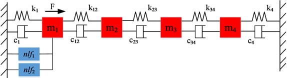
System parameters:

$M =$ [1, 0, 0, 0; 0, 2, 0, 0; 0, 0, 3, 0; 0, 0, 0, 5];

$C =$ [10, –5, 0, 0; –5, 10, –5, 0; 0, –5, 10, –5; 0, 0, –5, 10];

$K =$ [1000, –500, 0, 0; –500, 1000, –500, 0; 0, –500, 1000, –500; 0, 0, –500, 1000].

The nonlinear elements between m1 and ground are ‘cubic stiffness’, ${n l f}_{1}$ and ‘gap with end stiffness’ ${n l f}_{2}$ :

{n l f}_{1} = 1.7 e 5 \times {x_{1}}^{3},

{n l f}_{2} = \{\begin{array}{l} 0, & |x_{1}| < 0.008, \\ 2.3 e 2 \times (|x_{1}| - 0.008) ∙ s i g n (x_{1}), & |x_{1}| \geq 0.008 . \end{array}

The sinusoidal excitation is applied at DOF1. The system is linear under small excitation, while the nonlinearities appear when the excitation gets big enough.

The simulation tests are performed using harmonic force with frequency 2 Hz, Fig. 2. The FRFs obtained from 0.1 N amplitude harmonic force are taken as linear FRFs of system. For the nonlinear FRFs the force amplitude is stepped up to10 N. The simulation is performed with functions in a nonlinear MATLAB toolbox [9].

Fig. 2Linear and Nonlinear FRF H11

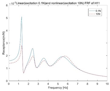
Fig. 3Sum of NLN of different DOFs

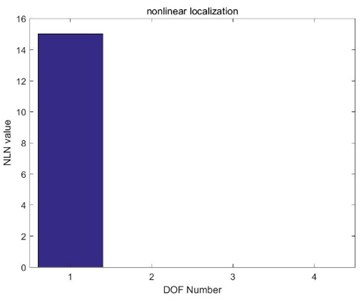
Fig. 4Comparison of calculated and fitted DF

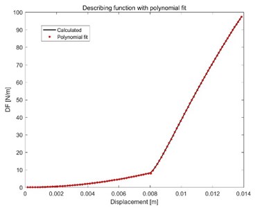
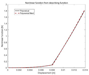
Fig. 5Comparison of theoretical and fitted nlf

From Fig. 3 it is found that the nonlinearities only exist between DOF1 and ground. By using measured FRF the describing function of system nonlinearities can be calculated by Eq. (9) and is shown in Fig. 4 (black). By observing, a turning point can obviously be found at the displacement 0.008 [m]. Polynomial fitting in interval [0, 0.008] and [0.008, $+ \infty$ ] is made with degrees 3 and 5, respectively. The polynomial fitted DF curve is obtained and shown in Fig. 4 (red). For the convenience of display, all values of displacement are multiplied by 1e+3. The polynomial coefficients, ${[c}_{n}, c_{n - 1}, \dots, c_{1}]$ , for each part are:

{c o e f}_{d f 1} = [- 0.0001, 0.1279, - 0.0008, 0.0003], 0 < A < 0.008,

{c o e f}_{d f 2} = 1 . e 3 * [- 0.0000, 0.0006, - 0.0146, 0.1695, - 0.9586, 2.0955], A \geq 0.008 .

Dividing ${c o e f}_{d f 1}$ and ${c o e f}_{d f 2}$ by the corresponding transform coefficients from Eq. (17), the polynomial coefficients for nonlinear force expressions are found. The comparison of fitted (red) and theoretical (black) nonlinear force functions is shown in Fig. 5:

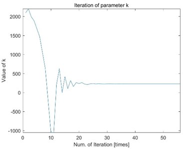
{c o e f}_{n l f 1} = [- 0.0001, 0.1706, - 0.0009, 0.0003], 0 < x < 0.008,

{c o e f}_{n l f 2} = 1 . e 3 * [- 0.0000, 0.0010, - 0.0215, 0.2260, - 1.1293, 2.0955], x \geq 0.008 .

By observing Fig. 5, when $0 < x < 0.008$ , the expression of force should be in the form of $n l f (x) = a_{3} \times x^{3}$ and the corresponding theoretical describing function, with parameter $a_{3}$ , is $d f (A) = a_{3} \times {0.75 \times A}^{2}$ . Setting the difference between DF with $a_{3}$ and DF calculated as the FUN in $f m$ in search (FUN, $a_{3}$ ) of MATLAB and giving $a_{3}$ an initial value 1.706 $e 5$ , we can get the value of $a_{3}$ with accuracy, $a_{3} =$ 169687. The change of parameter $a_{3}$ with the number of iterations is shown in Fig. 6. As it’s a pure cubic stiffness in the first interval, the nonlinearities could be a combination of a cubic stiffness and a nonlinearity with gap. Compare the values of fitted $n l f$ in Fig. 5 and $169687 \times x^{3}$ $(x \geq 0.008)$ . The guess for the nonlinear force is $n l f (x) = 169687 \times x^{3} + k (x - 0.008)$ . Similar to parameter $a_{3}$ , we do the parameter fitting using fminsearch. Give an initial value $1 e 3 ∙ 2.0955$ and parameter $k$ stays at the value $k =$ 228.0690 after iterations.

Fig. 6Iteration of parameter a3

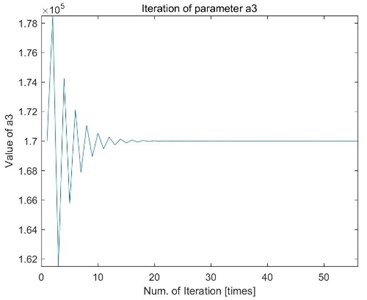
Fig. 7Iteration of parameter k

4. Conclusions

Identification of nonlinear system is considered by the inversion of describing functions. The method in this paper reduces the difficulty but improves the accuracy of nonlinear system identification. Thanks to the broad applicability of polynomial fitting, the polynomial inversion method should work out well for most situations in which the nonlinearities are in-dependent of frequency. The result of the illustrative example shows that this method is capable to identify the nonlinear systems with acceptable accuracy.

References

Kerschen G., et al. Review: past, present and future of nonlinear system identification in structural dynamics. Mechanical Systems and Signal Processing, Vol. 20, Issue 3, 2006, p. 505-593.

Publisher
Noël J. P., Kerschen G. Nonlinear system identification in structural dynamics: 10 more years of progress. Mechanical Systems and Signal Processing, Vol. 83, 2017, p. 2-35.

Publisher
Tanrikulu O., et al. Forced harmonic response analysis of nonlinear structures using describing functions. AIAA Journal, Vol. 31, Issue 7, 1993, p. 1313-1320.

Publisher
Özer M. B., Özgüven H. N., Royston T. J. Identification of structural nonlinearities using describing functions and Sherman-Morrison method. Mechanical Systems and Signal Processing, Vol. 23, Issue 1, 2009, p. 30-44.

Publisher
Aykan M., Özgüven H. N. Parametric identification of nonlinearity in structural systems using describing function inversion. Mechanical Systems and Signal Processing, Vol. 40, Issue 1, 2013, p. 356-376.

Publisher
Jalali H., Bonab B. T., Ahmadian H. Identification of weakly nonlinear systems using describing function inversion. Experimental Mechanics, Vol. 51, Issue 5, 2011, p. 739-747.

Publisher
Zhongge Zhao, Chuanri Li, Kjell Ahlin, Huan Du Nonlinear system identification with the use of describing functions – a case study. Vibroengineering Procedia, Vol. 8, 2016, p. 33‑38.

Search CrossRef
Gelb A., Vander Velde W. E. Multiple-Input Describing Functions and Nonlinear System Design. McGraw-Hill, 1968.

Search CrossRef
Ahlin K. Toolbox for simulation and parameter identification of nonlinear mechanical systems. Proceedings of IMAC 25, 2007.

Search CrossRef

Cited by

Time Invariant Static Nonlinearities of the Dynamical Systems

Róbert Szabolcsi

(2022)

Microgrid Optimization Scheduling Based on Improved Genetic Annealing Algorithm

君张

(2020)

About this article

Received

25 April 2017

Accepted

29 April 2017

Published

30 June 2017

SUBJECTS

Mathematical models in engineering

DOI

https://doi.org/10.21595/vp.2017.18538

Keywords

nonlinear system

identification

describing function

polynomial inversion method

This is an open access article distributed under the Creative Commons Attribution License, which permits unrestricted use, distribution, and reproduction in any medium, provided the original work is properly cited.

Previous article in issue Previous Next article in issue Next

Research article

2019 11 28

Unknown input reconstruction in non-linear dynamical systems using homotopy optimization

R. Manikantan, Sayan Chakraborty, C. P. Vyasarayani

Research article

2018 02 15

Research and application of Volterra series theory in rolling bearing fault state feature extraction

Haitao Wang, Zhenya Kang, Lichen Shi, Kun Wang, Xiao Zhang

Research article

2017 10 21

A stochastic surrogate model for time-variant reliability analysis of flexible multibody system

Linjie Kan, Jianguo Zhang, Qian Wang

Research article

2016 10 07

Nonlinear system identification with the use of describing functions – a case study

Zhongge Zhao, Chuanri Li, Kjell Ahlin, Huan Du

H. Du, Z. Li, and K. Ahlin, “On the inversion of describing functions in nonlinear system analysis,” Vibroengineering PROCEDIA, Vol. 12, pp. 172–177, Jun. 2017, https://doi.org/10.21595/vp.2017.18538

Copy Extrica

Copied to clipboard!

TY  - JOUR
DO  - 10.21595/vp.2017.18538
UR  - https://doi.org/10.21595/vp.2017.18538
TI  - On the inversion of describing functions in nonlinear system analysis
T2  - Vibroengineering PROCEDIA
AU  - Li, Zhiqiang
AU  - Du, Huan
AU  - Ahlin, Kjell
PY  - 2017
DA  - 2017/06/30
PB  - JVE International Ltd.
SP  - 172-177
VL  - 12
SN  - 2345-0533
ER  - 

Copy Ris

Copied to clipboard!

@article{Li_2017,
	doi = {10.21595/vp.2017.18538},
	url = {https://doi.org/10.21595/vp.2017.18538},
	year = 2017,
	month = {jun},
	publisher = {{JVE} International Ltd.},
	volume = {12},
	pages = {172--177},
	author = {Zhiqiang Li and Huan Du and Kjell Ahlin},
	title = {On the inversion of describing functions in nonlinear system analysis},
	journal = {Vibroengineering {PROCEDIA}}
}

Copy Bibtex

Copied to clipboard!

[1]Z. Li, H. Du, and K. Ahlin, “On the inversion of describing functions in nonlinear system analysis,” Vibroengineering PROCEDIA, vol. 12, pp. 172–177, Jun. 2017, doi: 10.21595/vp.2017.18538.

Copy IEEE

Copied to clipboard!

Li, Zhiqiang, Huan Du, and Kjell Ahlin. “On the Inversion of Describing Functions in Nonlinear System Analysis.” Vibroengineering PROCEDIA 12 (June 30, 2017): 172–77. https://doi.org/10.21595/vp.2017.18538.

Copy Chicago

Copied to clipboard!

On the inversion of describing functions in nonlinear system analysis

Abstract

1. Introduction

2. Theory

2.1. Describing function method

2.2. Polynomial inversion method

3. An illustrative example

4. Conclusions

References

Cited by

About this article

Related Articles