Single universal dimensionless specific energy curves for trapezoidal and circular shaped open channels

Tiruneh, Ababu T.

doi:10.21595/mme.2025.24850

Mathematical Models in Engineering

Browse Journal

Submit article

Published: September 29, 2025

Check for updates

Single universal dimensionless specific energy curves for trapezoidal and circular shaped open channels

Ababu T. Tiruneh¹

¹University of Eswatini, Department of Environmental Health Science, P.O. Box 369, Mbabane, Eswatini

Cite the article Download PDF

Downloads 172

Abstract

Trapezoidal and circular channels are commonly employed as conveyances of open channel flow in irrigation canals, for storm and wastewater drainage and at times for transporting raw water. Open channel flow problems in such cross sections typically involve determination of alternate depths, critical depths and specific energy that require solving equations for which explicit solutions are difficult to obtain. This paper demonstrates the development of a solution for such problems through the use of single universal dimensionless specific energy-depth curves for each of the trapezoidal and circular shaped channels. The dimensionless curves are demonstrated to be simple to develop and use and can be adapted for wide range of user environments. Simulation of the graphical solution over broader range of flows and dimensionless depths of flow shows that the solution is reasonably accurate with percentage error of estimation of depth varying between 0 and 4 % with mean percentage error of 1.1 % for trapezoidal shaped channels and 1.2 % for circular shaped channels. Further application examples have been provided that show that the proposed graphical procedure can achieve results that are within close range of the precision of results obtained using numerical methods.

Single universal dimensionless specific energy curves for trapezoidal and circular shaped open channels

Highlights

Single universal dimensionless specific energy curves have been developed for both trapezoidal and circular shaped channels.
The dimensionless curves can be used for the graphical determination of alternate depths as well as critical depth of flow in both trapezoidal and circular shaped channels.
The proposed graphical precoedure is an improvement over existing graphical methods that require dawing a dsicrete number of curves into a single plotting space.
The graphical method does not require interpolation among discerete number of curves as in the existing graphical methods. It is a continuous curve that is applicable for all gemoetric and flow condiitons.
The method used in developing the single universal dimensionless curve is a general procedure that can be similarly used to solve other types of hydraulic problems such as determination of normal depth of flow in open channels or graphical determination of friction factor in pipe flows.

1. Introduction

Trapezoidal and circular shaped open channels are commonly constructed in irrigation channels, in storm water drainage or as conduits for transmission of raw water sources [1]. Flow conditions in the regular trapezoidal and circular channels are relatively easy to establish and these channels are also convenient for construction in the form of the stable bank slopes provided by trapezoidal channels and the easier casting of circular shaped conduits [2]. Circular shaped channel cross sections are used as open channel flow conduits in hydraulic, irrigation and agricultural engineering applications because of their excellent hydraulic properties and convenient construction. Circular shaped sewer cross sections are also used in sewer systems because of their high discharge capacity, low rate of sedimentation at low flows and greater capacity to withstand compressive overburden loads [3-5]. Trapezoidal control sections are used to control the depths upstream in a channel so that normal water depth is maintained and chocking conditions are avoided. When provided at the entrances of drop structures and chutes, trapezoidal control sections prevent the development of shear force that can cause erosion of the channel. Trapezoidal control sections are also provided at the inlets of inverted siphons to prevent drop in water surface below the crown of the inverted siphon that causes air locks and flow stoppage, a situation that arises during low flow periods when the flow in the sewer is less than the design discharge [6].

Open channel flows are commonly analysed for alternate, normal and critical depths as part of engineering design that involve solving flow related problems [7]. Open channel flow problems such as determining the energy loss involving hydraulic jump can be solved by writing the specific energy equation together with the specific force equation. The specific energy can be interpreted as the sum of the potential energy and kinetic energy of fluid with respect to the bottom of the channel [8]. The specific energy at a given channel section is given as:

1

E = y + \frac{α Q^{2}}{2 g A^{2}},

where, $E$ is the specific energy, $y$ is the depth of flow, $Q$ is the discharge through the channel, $A$ is the cross sectional area of the channel, g is acceleration due to gravity and $α$ is the energy coefficient at the section. Explicit solutions for alternate, normal and critical depths in trapezoidal and circular channels are difficult to obtain. The equations needed for determination of normal and critical depths in trapezoidal and circular channels are either fifth or six degree polynomials (for trapezoidal channels) where algebraic solutions are impossible to obtain, or, are transcendental equations that are in implicit form (for circular channels) where explicit solutions are difficult to establish. As a result, engineers commonly use iterative techniques that are based on numerical approximation methods such as the Newton-Raphson method that are solved either manually or using computer programs/software. As a direct solution alternative, several methods have been developed by researchers for finding the determination of alternate and critical depths of flow in trapezoidal and circular channels. Most of the methods that were recently developed are based on numerical procedures [7]. Such numerical methods range from analytical solutions involving inversion problems to iterative procedures or even methods involving machine learning algorithms.

Das [9] used solutions of quadratic and cubic equations for determination of alternate depths and sequent depths in trapezoidal, rectangular and triangular channels. Swamee and Rathie developed exact solutions (complex equations as infinite series) for normal depth in rectangular, trapezoidal and circular sections using the Chezy and Manning’s equations [10]. Swamee and Rathie [11] further developed exact solutions for critical depth in trapezoidal section in the form of fast converging infinite series but the computation is complicated if higher accuracy is to be achieved [12]. Wong and Zhou developed implicit analytical equations and used Microsoft Excel spreadsheet to determine critical and normal depths for triangular, trapezoidal parabolic and circular channels using analytical equations and Goal seek function for root solving [13]. Kanani et al. developed a general and accurate method for determining critical depth for any prismatic and non-prismatic open channel cross sections using evolutionary genetic algorithms but may be impractical for designers to use [14]. Mohammed et al. [15] used dimensional analysis to propose analytical equation for measuring critical and normal depths in circular channels using dimensionless parameters representing the water depth as the dependent variable and another dimensionless variable which is a function of the flow rate and pipe diameter as the independent variable. The resulting error of prediction of normal and critical depths of flow were reportedly lower than the percentage errors reported by previous researchers.

Further examples of the development of numerical methods for determining critical depth in open channels have been given by a number of authors [1], [2], [7], [11], [16], [17]. These methods claim to be explicit. However, they tend to be complex in terms of the analytical techniques used for their development or the procedure used in the determination of depths of flow. This is not, however, to suggest that these methods are not competent. On the contrary, numerical methods are better in terms of their numerical precision compared to the graphical methods. However, familiarization with the numerical techniques as well as with the procedure required to use them are needed and this may not be always easy for all range of users interested in solving open channel flow related problems.

The use of graphical method was more common prior to the advent of modern computers in hydraulic engineering applications and for solving open channel flow related problems. Graphical procedures for solving open channel flow related problems have been established in the past that involve using plotted graphs or graphs that are combined with semi analytical/numerical procedures [18-21]. Babaeyan-Koopaei [22] proposed dimensionless graphs for the determination of normal depths for rounded-bottom triangular, parabolic and rounded coner rectangular cross sections. However, these shapes have limited used for practical designs although the graphical development of the methods is relatively easy to establish [23], [24]. Graphical solutions for trapezoidal channels sections used as control structures suggested by USBR [25] are specifically used for small discharges less than 2.83 m³/sec and specific values of channel bottom width and side slopes. The design of the control notch even while using this graphs still requires a trial and error procedure [6].

With the present day power of computers and the availability of software programs that merely require inputting of needed data to solve open channel flow related problems, it may not be easy to make a case for graphical methods for solving open channel flow problems. However, graphical methods are fast and easy to use and they do not need sophisticated software programs for their implementation. For many applications, graphical methods can yield results in simple steps with acceptable precision.

Methods for analysing open channel flow related problems using dimensionless variables have been developed for different channel cross sections. In this respect, trapezoidal and circular channels are somewhat difficult to analyse in terms of dimensionless variables. However, there were attempts made in the past of such analyses using dimensionless curves. One example of the use of dimensionless graphs for determination of alternate and critical depths in circular and trapezoidal open channels is shown by Jeppson [26]. However, the dimensionless curves are not a single curve. For both the trapezoidal and circular shaped channels, several dimensionless graphs have to be drawn for a different combination of discharge, side slope, channel base width and pipe diameter. Furthermore, the dimensionless graphs so developed involve a discrete number of curves and cannot cover the entire continuum of the combination of such variables mentioned. In this respect, it would be useful to examine the graphs provided in the book by Jepson [26] on page 133 to observe the number of discrete curves that have to be drawn in order to use the dimensionless graphs. These graphs are shown in Fig. 1 and Fig. 2 for trapezoidal and circular channels respectively. The graphs in these figures indicate the necessity of drawing several dimensionless curves in the plotting space which makes such plotting cumbersome. In addition, since there is only discrete number of curves that are drawn and do not cover the entire continuum of variation of flow conditions, there is a need for interpolation when the dimensionless parameters in the graphs lie in between the curves. This can give rise to errors.

Fig. 1Dimensionless specific energy diagrams for trapezoidal channels [26]

Fig. 2Dimensionless specific energy diagrams for circular channels [26]

Determination of alternate depths of flow in stilling basin design that employ hydraulic jumps for energy dissipation uses iterative techniques for trapezoidal and triangular channel cross sections whereas straightforward numerical solution is possible for rectangular channel sections [8]. In addition simpler graphical procedures are available for rectangular channel sections for such problems of erosion control. Trapezoidal channel cross-sections on the other hand do not easily lend themselves to simple graphical solution because of the channel geometries that necessitate drawing several, discrete number of curves in a single plotting space.

While methods for solving open channel flow problems using a single dimensionless curve has been developed for parabolic shaped open channels [26], to the author’s knowledge, there is no such single dimensionless curve that is developed either for trapezoidal or circular shaped open channels.

2. Objective of the proposed graphical method

The objective of the graphical method proposed in this paper is to solve open channel flow related problems involving specific energy in trapezoidal and circular shaped channels through the use of a single universal dimensionless curves. The use of singe dimensionless curve for solve open channel flow related problems in such channel cross sections facilitates simple graphical method of determining the alternate and critical depths of flow without resorting to the use of complicated numerical procedures that often involve iterative steps. By developing a single dimensionless curve, the need for drawing several dimensionless curves that are crowded into a single graph is avoided. Drawing multiple dimensionless curves in a single graph makes reading from the graphs difficult. In addition, the graphs are drawn for discrete combination of flow an channel cross section parameters and as such do not cover the entire continuum of variation of such flow and channel cross section parameters. On the other hand, the development of a single universal dimensionless curve eliminates the need for interpolation or guessing that has to be made in between these discrete number of curves for which curves are not drawn. In addition, the fact that there is only a single universal curve makes the plotting space wider and facilitates more accurate reading from the curves. The use of a single universal dimensionless curve has also the objective of providing solutions to all types of flow related problems arising in trapezoidal and circular channel cross sections that are applicable to variations in flow, channel cross section slope, flow depth, etc.

3. Methods

The graphical method of solving open channel flow related problems in circular and trapezoidal shaped channels based on the use of single, dimensionless curves is presented below. The methodology presented below starts with trapezoidal shaped open channels and repeats the procedure also for circular shaped open channels. The specific energy equations are formulated first for each shape, and a method is provided for the expression of depth of flow and specific energy in dimensionless forms. Finally, a graphical procedure is presented that allows the determination of either water depth and/or specific energy of flow as the case may be.

3.1. Trapezoidal channels

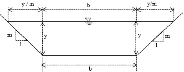
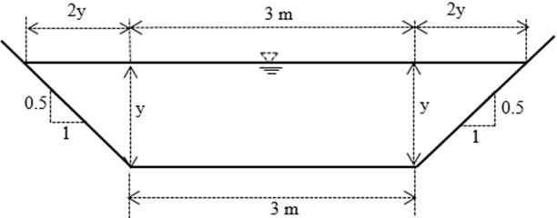
Fig.3 shows a cross section of a trapezoidal shaped open channel having bottom width $b$ , side slopes $H$ : $V$ of 1: $m$ . For a given discharge, $Q$ , the specific energy, $E$ , can be written as:

2

E = y + \frac{V^{2}}{2 g} = y + \frac{Q^{2}}{2 g A^{2}} = y + \frac{Q^{2}}{2 g {(b y + \frac{y^{2}}{m})}^{2}} = y + \frac{Q^{2}}{2 g b^{2} y^{2} {(1 + \frac{y}{b m})}^{2}},

where $A$ is the cross sectional area, $Q$ is the discharge, $v$ is the average velocity, $y$ is the depth of flow.

Introducing the dimensionless depth $y_{u}$ and specific energy, $E_{u}$ i.e.:

3

y_{u} = \frac{y}{m b}, E_{u} = \frac{E}{m b} .

The significance of introducing the dimensionless depth $y_{u}$ and specific energy, $E_{u}$ as given by Eq. (3) lies in the fact that subsequent graphs that are plotted based on these dimensionless variables can be universally used for any trapezoidal channel geometry as these variables are independent of any particular channel geometry.

Eq. (2) can now be written as:

4

E_{u} = y_{u} + (\frac{Q^{2}}{g b^{5} m^{3}}) . (\frac{1}{2 {y_{u}}^{2} (1 + y_{u})^{2})}) .

Fig. 3Trapezoidal channel with bottom width b, depth y and side slopes 1H: mV

Defining further a dimensionless quantity, $θ^{3}$ such that:

5

θ^{3} = \frac{Q^{2}}{g b^{5} m^{3}} .

The meaning of $θ^{3}$ is may be expressed as the dimensionless critical depth, $y_{R C}$ , of trapezoidal channel with large width b (or equivalent rectangular channel of width $b$ ). For a discharge per unit width $q = Q / b$ , $θ^{3}$ can be expressed as:

6

θ^{3} = \frac{Q^{2}}{(g b^{5} m^{3})} = \frac{q^{2}}{(g b^{3} m^{3})} = {[{(\frac{q^{2}}{g})}^{(1 / 3)} (\frac{1}{b m})]}^{3} = {(\frac{y_{R C}}{b m})}^{3} .

So that:

7

θ = \frac{y_{R C}}{b m} .

Eq. (4) can now be written incorporating the expression for $θ^{3}$ given by Eq. (5) as follows:

8

E_{u} = y_{u} + \frac{θ^{3}}{2 {y_{u}}^{2} (1 + y_{u})^{2}} .

The importance of introducing the dimensionless critical depth $θ$ will become apparent as the dimensionless graph developed will make use of this dimensionless parameter in drawing a slope line that intersect the dimensionless curve and from which the dimensionless alternate depths of flow are read.

Rearranging Eq. (8) further gives:

9

\frac{1}{θ^{3}} (E_{u} - y_{u}) = \frac{1}{2 {y_{u}}^{2} (1 + y_{u})^{2}} .

Adding $y_{u}$ to both sides of Eq. (9) and further rearranging:

10

\frac{E_{u}}{θ^{3}} + (\frac{(θ^{3} - 1)}{θ^{3}}) y_{u} = y_{u} + \frac{1}{2 {y_{u}}^{2} (1 + y_{u})^{2}} .

Defining a dimensionless specific energy function for channels with trapezoidal shape cross sections, $β$ such that:

11

β = \frac{E_{u}}{θ^{3}} + (\frac{(θ^{3} - 1)}{θ^{3}}) y_{u} = y_{u} + \frac{1}{2 {y_{u}}^{2} (1 + y_{u})^{2}} .

The variable $β$ is the dimensionless specific energy function for channels with trapezoidal shape cross section. It is purely dependent only on the dimensionless depth of flow, $y_{u}$ as Eq. (11) shows and can therefore be determined once the $y_{u}$ is known. This dimensionless specific energy function, $β$ , is one of the variables that is needed for plotting the dimensionless specific energy curve as it mentioned below.

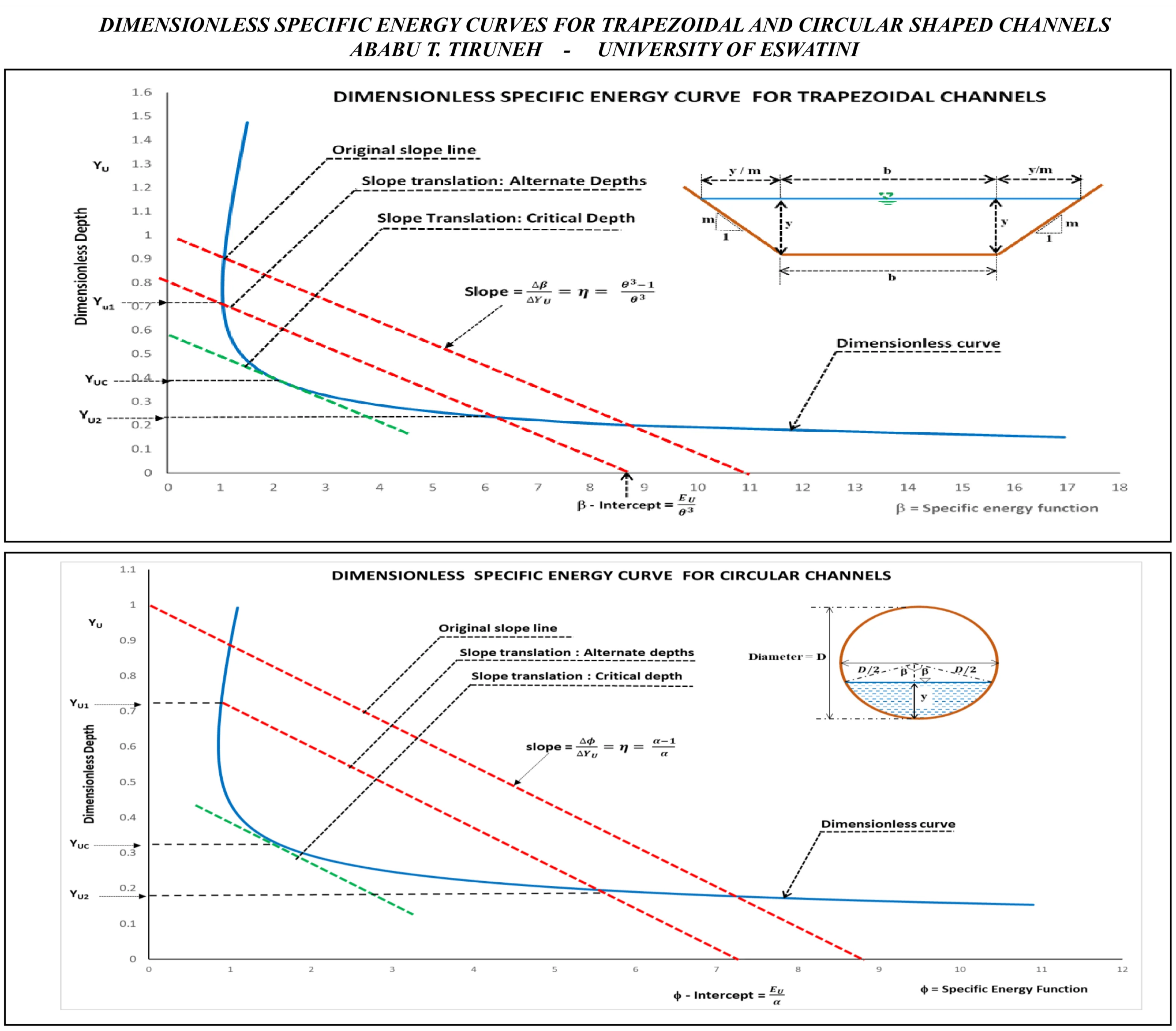
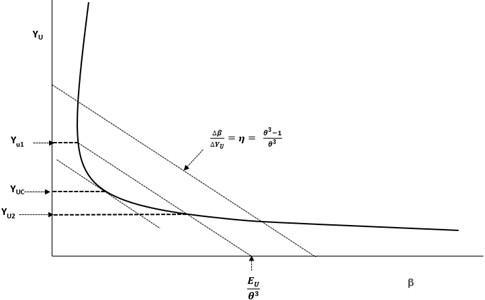
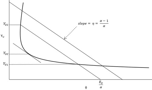
A dimensionless graph can now be constructed using Eq. (11) with the dimensionless specific energy function $β$ plotted on the $x$ -axis and the dimensionless depth $y_{u}$ plotted on the $y$ axis. An illustration of such graph is shown in Fig. 4.

From Eq. (11), it is apparent that for a given specific energy $E_{u}$ expressed in dimensionless form, a line can be defined with a slope $η$ such that:

12

\frac{(β_{2} - β_{1})}{(y_{u 2} - y_{u 1})} = \frac{Δ β}{Δ y_{u}} = \frac{(θ^{3} - 1)}{θ^{3}} = η .

The introduction of a slope line with a slope $η$ as defined by Eq. (12) is useful because when this slope line is made to intersect the dimensionless specific energy function $β$ versus dimensionless depth of flow $y_{u}$ curve, it uniquely relates the alternate depths and the specific energy for any given flow condition in trapezoidal channels. In other words, by passing this slope line through the dimensionless curve at a particular specisfic energy value, the alternate depths can be determined and vice versa.

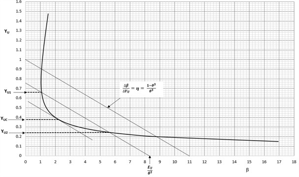
The use of the dimensionless $(β - y_{u}$ ) curve for solving open channel flow related problems is now evident from examination of Fig. 4 that shows the slope, $η$ , alternate depths $y_{u 1}$ and $y_{u 2}$ and the critical depth $y_{c}$ . For example, if the upstream depth $y_{1}$ is given (and hence $y_{u 1}$ ), the downstream dimensionless depth $y_{u 2}$ can be determined by passing a line $η$ through $y_{u 1}$ and intersecting the $β$ - $y_{u}$ curve at the point $y_{u 2}$ . Likewise, if the specific energy $E$ (and hence $E_{u}$ ) is given while both alternative depths, $y_{u 1}$ and $y_{u 2}$ are unknown, these depths can be determined by passing the $η$ -line through the $β$ -intercepts, $E_{u} / θ^{3}$ , and intersecting the $β$ - $y_{u}$ curve at the points $y_{u 1}$ and $y_{u 2}$ . This is illustrated in Fig. 4.

Fig. 4Dimensionless graph (β-yu) for trapezoidal channels

To determine the critical depth, differentiating the expression given by Eq. (11) with respect to $y_{u}$ gives:

13

\frac{d β}{d y_{u}} = (\frac{1}{θ^{3}}) \frac{d E_{u}}{d y_{u}} + \frac{(θ^{3} - 1)}{θ^{3}} .

Since at the critical depth $\frac{d E_{u}}{d y_{u}} = \frac{d E}{d y} =$ 0:

14

\frac{d β}{d y_{u}} = \frac{(θ^{3} - 1)}{θ^{3}} .

Eq. (14) indicates that the critical depth can be determined by sliding the $η$ -line until it becomes tangent to the $β$ - $y_{u}$ curve. A further numerical solution may become possible for determining the critical depth from the graphical solution since there is a unique relationship between the given slope, $η$ , and the dimensionless depth of flow $y_{u}$ as the following relationship is apparent from Eq. (11) and Eq. (14):

\frac{d β}{d y_{u}} = \frac{(θ^{3} - 1)}{θ^{3}} = η = \frac{d (y_{u} + \frac{1}{2 {y_{u}}^{2} (1 + y_{u})^{2}})}{d y_{u}} .

The above ordinary differential equation (ODE) can be solved numerically to determine the critical depth. Alternatively, the five degree polynomial equation that results by differentiating the right side of the above equation can also be solved numerically.

The steps needed for developing the dimensionless curve and using the graphical method outlined above is given below while the results of simulation of the graphical solution for broader range of discharge values and dimensionless depths of flow are provided in Section 3 under the Results sections. Furthermore, application of the dimensionless specific energy curve for trapezoidal shaped channels is further demonstrated with a worked example provided in Section 3 under Application Examples.

3.2. Procedure for developing and using the universal dimensionless specific energy curve for trapezoidal channel cross sections.

The dimensionless curve for trapezoidal channel cross sections on which the proposed graphical method is based can be developed using graphical plotting software such as Microsoft Excel. The procedure for using the graph can also be implemented using Microsoft Excel. Alternatively, the graph can be printed on paper and used manually. The advantage of using the Microsoft Excel software directly is because of the zooming large capability on the graph that allows a more accurate reading from the graphs as well as the ability to change the plotting range of $β$ and $y_{u}$ in order to suit a particular problem at hand. On the other hand, the manual method on a printed graph can also be used for specific ranges of $β$ and $y_{u}$ values that are plotted on larger scale in order to allow reasonably accurate prediction of alternate depths or specific energy values. The procedure below lists the steps needed in developing the dimensionless specific energy curve outlined above as well as in using the graph to solve a particular problem.

1) Plotting the dimensionless curve: The graph of the dimensionless specific energy function $β (y_{u})$ is plotted on the $x$ -axis against the dimensionless depth of flow $y_{u}$ on the $y$ -axis using the Microsoft Excel graph and as shown in Fig. 4. For a given dimensionless depth of flow $y_{u}$ , the corresponding $β (y_{u})$ value is calculated using Eq. (11) which is reproduced below:

β (y_{u}) = y_{u} + \frac{1}{2 {y_{u}}^{2} (1 + y_{u})^{2}} .

2) For problems of determining alternate depths given specific energy: This problem involves the determination of alternate depths of flow from a given specific energy of flow. For a given problem of flow in trapezoidal cross section channel in which the flow rate is given as $Q$ , the specific energy is given as $E$ , the bottom width of the trapezoidal cross section given as b and the side slope of 1H: mV, the dimensionless specific energy $E_{u}$ is calculated as:

E_{u} = \frac{E}{m b} .

3) Determination of the $θ^{3}$ value: The cube of the dimensionless $θ$ value which is the dimensionless critical depth of equivalent rectangular cross section channel with a width b and carrying a discharge $Q$ is calculated as follows:

θ^{3} = \frac{Q^{2}}{g b^{5} m^{3}} .

4) Determination of the slope line, $η$ : The slope, $η$ , of the line connecting the alternate depths of flow that have the same specific energy in the dimensionless depth versus specific energy curve of trapezoidal cross section channels is calculated as follows:

η = \frac{Δ β}{Δ y_{u}} = \frac{(θ^{3} - 1)}{θ^{3}} .

5) Drawing of the slope line on the dimensionless curve: The line having a slope $η$ determined in step 4 above is drawn on the dimensionless curve developed in step 1 above. This line is shown in Fig. 4 as a dotted line and is labelled with slope, $η$ . The line is drawn for example by setting the vertical $y_{u}$ value to one and the horizontal $β$ value to $η$ as the formula for $η$ given in step 4 above shows.

6) Determination of the $β$ -intercept: The $β$ -intercept on the dimensionless curve is the point on the horizontal $β$ -axis at which the slope line determined in step 5 above will eventually pass and intersects the $β$ -axis. This point is determined using the formula:

β_{i n t e r c e p t} = \frac{E_{u}}{θ^{3}} .

7) Determination of the dimensionless alternate depths, $y_{u 1}$ and $y_{u 2}$ : The dimensionless alternate depths $y_{u 1}$ and $y_{u 2}$ are determined by copying the slope line drawn in Step 5 above and moving the line in parallel (so that the slope $η$ remains the same) until the line passes through the $β$ -intercept on the $β$ -axis as determined in Step 6 above. This line is also shown in Fig. 4. The intersection of the slope line with the dimensionless $β$ - $y_{u}$ curve will give the values of the dimensionless alternate depths $y_{u 1}$ and $y_{u 2}$ . These values are read from the vertical $y_{u}$ axis by extending horizontal lines from the intersection points towards the vertical $y_{u}$ axis. In order to help with more accurate reading of the $y_{u}$ values, the graph can be zoomed large on Microsoft Excel graph. Adequate number of major and minor grid lines can also be drawn on the graph using Microsoft Excel graph to enable better reading of the dimensionless alternate depth values from the graph.

8) Determination of the alternate depths of flow $y_{1}$ and $y_{2}$ : Once the dimensionless alternate depths $y_{u 1}$ and $y_{u 2}$ are determined as shown in Step 7 above, the corresponding alternate depths of flow, $y_{1}$ and $y_{2}$ are determined from the following formula:

y_{1} = y_{u 1} (m b), y_{2} = y_{u 2} (m b) .

9) Determination of the critical depth of flow, $y_{c}$ : In order to determine the critical depth, the slope line is copied and moved in parallel until it becomes tangent to the dimensionless $β$ - $y_{u}$ curve. This is shown in Fig. 4. The corresponding dimensionless critical depth $y_{u c}$ is read from the tangent point by extending a horizontal line towards the vertical $y_{u}$ axis. The graph can be zoomed large by using the Microsoft Excel zooming tool bar. The zooming large capability of Microsoft excel will help in locating the tangent point on the dimensionless curve at which the slope line touches the graph as well as for reading the corresponding dimensionless critical depth $y_{u c}$ more accurately from the vertical $y_{u}$ axis. Once the dimensionless critical depth $y_{u c}$ is determined, the corresponding critical depth $y_{c}$ is determined using the formula:

y_{c} = y_{u c} (m b) .

10) For problems of given depth of flow and determining the corresponding alternate depth: For open channel flow problems in which a depth of flow $y_{1}$ is given and the corresponding alternate depth $y_{2}$ is to be determined, first the corresponding dimensionless depth $y_{u 1}$ of the given depth $y_{1}$ is calculated as:

y_{u 1} = \frac{y_{1}}{m b} .

Next, the slope line is determined using Steps 3, 4 and 5 above. This slope line is copied and moved in parallel until it intersects the dimensionless $β$ - $y_{u}$ curve at $y_{u 1}$ . The dimensionless alternate depth $y_{u 2}$ is read from the other intersection point of the slope line and the dimensionless curve. The corresponding alternate depth $y_{2}$ is calculated from:

y_{2} = y_{u 2} (m b) .

3.3. Circular channels

For flow in open channels of circular shaped cross section with diameter $D$ in which the depth of flow is $y$ as shown in Fig. 5, the specific energy is formulated as follows:

15

E = y + \frac{v^{2}}{2 g} = y + \frac{Q^{2}}{(2 g A^{2})} = D (\frac{1 - c o s β}{2}) + \frac{8 Q^{2}}{g D^{4} (β - s i n β c o s β)^{2}} .

Fig. 5Cross sectional view of open channel flowing partially full in a circular shaped channel

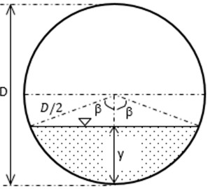
In Eq. 15, $β$ is the angle between the vertical line and the line connecting edges of the water surface line with the centre of the circle as shown in Fig. 5. Defining the dimensionless depth, $y_{u}$ and dimensionless specific energy $E_{u}$ for circular channels given by Eq. (16):

16

y_{u} = \frac{y}{D} = \frac{1 - \cos β}{2}, E_{u} = \frac{E}{D} .

The importance of introducing the dimensionless depth and specific energy values as given by Eq. (16) for circular shaped channels is the same as that of trapezoidal shaped channels of the ability to plot and use dimensionless graphs based on these dimensionless variables that can be used to solve flow problems irrespective of the particular channel geometries specified in the problems.

Eq. (15), can now be rewritten in terms of $y_{u}$ and $E_{u}$ as follows:

17

E_{u} = y_{u} + \frac{8 Q^{2}}{g D^{5} (β - s i n β c o s β)^{2}} .

Furthermore, defining a dimensionless quantity, $α$ , such that:

18

α = \frac{8 Q^{2}}{g D^{5}} .

The dimensionless variable $α$ for circular shaped channels can be analogously defined similar to the definition the dimensionless equivalent critical depth of rectangular channel with the same flow rate $Q$ as the trapezoidal channel: $θ = y_{R C} / b m$ . This dimensionless parameter is shown below to be a linear function of the equivalent critical depth of a circular channel flowing full with the same flow rate $Q$ and full flow velocity $v$ , i.e., $α = f (y_{c c} / D)$ . From Eq. (18):

\frac{8 Q^{2}}{g D^{5}} = a (\frac{V^{2}}{g D}),

where $a$ is a constant and $V$ is the velocity of flow when the channel is flowing full. Consider another circular channel of diameter $d$ and in which the flow rate is $V$ when flowing full so that $d$ is the critical depth of flow, i.e. $d = y_{c c}$ . It can be shown that:

y_{c c} = d = 2 (\frac{V^{2}}{g}) .

So that:

α = \frac{8 Q^{2}}{g D^{5}} = a (\frac{V^{2}}{g D}) = \frac{a}{2} (\frac{y_{c c}}{D}) .

Which shows $α$ to be a linear function of the relative critical depth of flow in a channel with the same flow rate and full flow velocity. The importance of introducing the dimensionless critical depth $α$ for circular channels will also become apparent as the dimensionless graph developed will make use of this dimensionless parameter in drawing a slope line that intersect the dimensionless curve and from which the dimensionless alternate depths of flow are read.

Eq. (17) can now be rewritten as:

19

\frac{E_{u}}{α} - (\frac{1}{α}) y_{u} = \frac{1}{(β - s i n β c o s β)^{2}} .

Adding the dimensionless depth $y_{u} = \frac{1 - c o s β}{2}$ given by Eq. (16) on both sides of Eq. (19) gives:

20

\frac{E_{u}}{α} + (1 - \frac{1}{α}) y_{u} = \frac{1 - c o s β}{2} + \frac{1}{(β - s i n β c o s β)^{2}} .

Defining a dimensionless specific energy function for channels with circular shape cross sections, $ϕ$ such that:

21

ϕ (y_{u}) = \frac{E_{u}}{α} + (\frac{α - 1}{α}) y_{u} = \frac{1 - c o s β}{2} + \frac{1}{(β - s i n β c o s β)^{2}},

β = c o s^{- 1} (1 - 2 y_{u}) .

The variable $ϕ$ is the dimensionless specific energy function for channels with circular shaped cross section. It is purely dependent only on the dimensionless depth of flow, $y_{u}$ as Eq. (21) shows since the angle $β$ is related to the dimensionless depth $y_{u}$ and can therefore be determined once the $y_{u}$ is known. This dimensionless specific energy function, $ϕ$ , for circular shaped channels is one of the variables that is needed for plotting the dimensionless specific energy curve as it mentioned below.

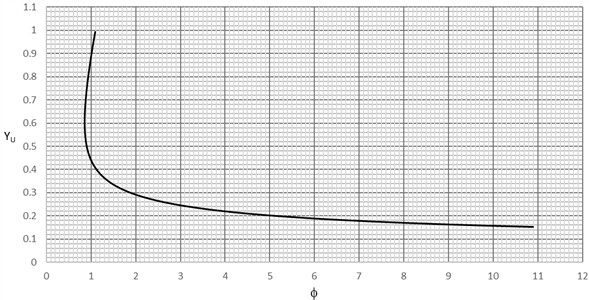
A dimensionless graph can now be constructed using Eq. (21) with the variable $ϕ$ plotted on the $x$ -axis and the dimensionless depth $y_{u}$ plotted on the $y$ axis. An illustration of such a graph is provided in Fig. 6. The similarity of the dimensionless equations and corresponding dimensionless graphs for the trapezoidal and circular shaped channels is now apparent.

From Eq. (21), as in the trapezoidal shaped channels, for a given specific energy $E_{u}$ expressed in dimensionless form, a line can be defined having a slope $η$ such that:

22

\frac{ϕ_{2} - ϕ_{1}}{y_{u 2} - y_{u 1}} = \frac{Δ ϕ}{Δ y_{u}} = η = \frac{α - 1}{α} .

The introduction of a slope line with a slope $η$ as defined by Eq. (22) for circular shaped channels is useful in a manner analogous to that of the trapezoidal channels because, when this slope line is made to intersect the dimensionless specific energy function $ϕ$ versus dimensionless depth of flow $y_{u}$ curve, it uniquely relates the alternate depths and the specific energy for any given flow condition in circular shaped channels. In other words, by passing this slope line through the dimensionless curve at a particular specific energy value, the alternate depths can be determined and vice versa.

In Fig. 6, if the upstream depth $y_{1}$ is given (and hence $y_{u 1}$ ), the downstream dimensionless depth $y_{u 2}$ can be determined by passing a line $η$ through $y_{u 1}$ and intersecting the $ϕ$ - $y_{u}$ curve at the point $y_{u 2}$ . Likewise, if the specific energy $E$ (and hence $E_{u}$ ) is given while both alternative depths $y_{u 1}$ and $y_{u 2}$ are unknown, these depths can be determined by passing the $η$ -line through the $β$ -intercept, $E_{u} / α$ and intersecting the $ϕ$ - $y_{u}$ curve at the points $y_{u 1}$ and $y_{u 2}$ .

To determine the critical depth, differentiating the expression in Eq. (21) with respect to $y_{u}$ gives:

23

\frac{d ϕ}{d y_{u}} = (\frac{1}{α}) \frac{d E_{u}}{d y_{u}} + (\frac{α - 1}{α}) d .

Sine at the critical depth $\frac{d E_{u}}{d y_{u}} = \frac{d E}{d y} =$ 0, Eq. (23) gives:

24

\frac{d ϕ}{d y_{u}} = (\frac{α - 1}{α}) .

Eq. (24) indicates that the critical depth can be determined by sliding the $η$ -line until it becomes tangent to the $ϕ$ - $y_{u}$ curve.

Fig. 6Dimensionless specific energy curve (ϕ-yu) for circular shaped channels

The steps needed for developing the dimensionless curve and using the graphical method outlined above for channels of circular cross section is given below while the results of simulation of the graphical solution for broader range of discharge values and dimensionless depths of flow are provided in Section 3 under the Results sections. Further application of the dimensionless specific energy curve for circular shaped channels is demonstrated with a worked example in Section 3: Application Examples.

3.4. Procedure for developing and using the universal dimensionless specific energy curve for trapezoidal channel cross sections

The dimensionless curve for circular shaped channel cross sections on which the proposed graphical method is based can also be developed using graphical plotting software such as Microsoft Excel as demonstrated above for trapezoidal channel cross sections. The procedure below lists the steps involved in developing the dimensionless specific energy curve of circular shaped channels outlined above and in using the graph to solve a particular problem.

1) Plotting the dimensionless curve: The graph of the dimensionless specific energy function for circular shaped channel, $ϕ (y_{u})$ , is plotted on the $x$ -axis against the dimensionless depth of flow, $y_{u}$ , on the $y$ -axis using the Microsoft Excel graph and as shown in Fig. 6. For a given dimensionless depth of flow $y_{u}$ , the angle $β$ and the $ϕ (y_{u})$ value are calculated using Eq. (16) and Eq. (21) which are reproduced below:

β = c o s^{- 1} (1 - 2 y_{u}),

ϕ (y_{u}) = \frac{1 - c o s β}{2} + \frac{1}{(β - s i n β c o s β)^{2}} .

2) For problems of determining alternate depths given specific energy: This problem involves the determination of alternate depths of flow from a given specific energy of flow. For a given problem of flow in circular cross section channel in which the flow rate is given as $Q$ , the specific energy is given as $E$ and the diameter of the cross section given as $D$ , the dimensionless specific energy $E_{u}$ is calculated as:

E_{u} = \frac{E}{D} .

3) Determination of the $α$ value: The $α$ value dimensionless parameter which is a linear function of the equivalent critical depth of a circular channel flowing full with the same flow rate $Q$ and full flow velocity $v$ . $α = f (\frac{y_{c c}}{D})$ is calculated as follows:

α = \frac{8 Q^{2}}{g D^{5}} .

4) Determination of the slope line, $η$ : The slope, $η$ , of the line, connecting alternate depths having the same specific energy in the dimensionless depth versus specific energy curve of circular cross section channels is calculated as follows:

η = \frac{α - 1}{α} .

5) Drawing of the slope line on the dimensionless curve: The line having a slope $η$ determined in step 4 above is drawn on the dimensionless curve developed in step 1 above. This line is shown in Fig. 6 as a dotted line and labelled with slope, $η$ . The line is drawn for example by setting the vertical $y_{u}$ value to one and the horizontal $ϕ$ value to $η$ as the formula for $η$ given in step 4 shows.

6) Determination of the $ϕ$ -intercept: The $ϕ$ -intercept on the dimensionless curve is the point on the horizontal $ϕ$ -axis at which the slope line determined in step 5 above will eventually pass and intersects the $ϕ$ -axis. This point is determined using the formula:

ϕ_{i n t e r c e p t} = \frac{E_{u}}{α} .

7) Determination of the dimensionless alternate depths, $y_{u 1}$ and $y_{u 2}$ : The dimensionless alternate depths $y_{u 1}$ and $y_{u 2}$ are determined by copying the slope line drawn in Step 5 above and moving the line in parallel (so that the slope $η$ remains the same) until the line passes through the $ϕ$ -intercept on the $ϕ$ -axis as determined in Step 6 above. This line is also shown in Fig. 6. The intersection of the slope line with the dimensionless $ϕ$ - $y_{u}$ curve will give the values of the dimensionless alternate depths $y_{u 1}$ and $y_{u 2}$ . These values are read from the vertical $y_{u}$ axis be extending horizontal lines from the intersection points towards the vertical $y_{u}$ axis. In order to help with more accurate reading of the $y_{u}$ values the graph can be zoomed large on Microsoft Excel graph. Adequate number of major and minor grid lines can also be drawn on the graph using Microsoft excel graph to enable better reading of the dimensionless alternate depth values from the graph.

8) Determination of the alternate depths of flow $y_{1}$ and $y_{2}$ : Once the dimensionless alternate depths $y_{u 1}$ and $y_{u 2}$ are determined as shown in Step 7 above, the corresponding alternate depths of flow, $y_{1}$ and $y_{2}$ are determined from the following formula:

y_{1} = y_{u 1} * D, y_{2} = y_{u 2} * D .

9) Determination of the critical depth of flow, $y_{c}$ : In order to determine the critical depth, the slope line is copied and moved in parallel until it becomes tangent to the dimensionless $ϕ$ - $y_{u}$ curve. This is shown in Fig. 6. The corresponding dimensionless critical depth $y_{u c}$ is read from the tangent point by extending a horizontal line towards the vertical $y_{u}$ axis. The graph can be zoomed large by using the Microsoft Excel zooming tool bar. The zooming large capability of Microsoft Excel can be used in order to more accurately locate the tangent point on the dimensionless curve at which the slope line touches the graph as well as for reading the corresponding dimensionless critical depth $y_{u c}$ more accurately from the vertical $y_{u}$ axis. Once the dimensionless critical depth $y_{u c}$ is determined, the corresponding critical depth $y_{c}$ is determined using the formula:

y_{c} = y_{u c} * D .

10) For problems of given depth of flow and determining the corresponding alternate depth: For open channel flow problems in which a depth of flow $y_{1}$ is given and the corresponding alternate depth $y_{2}$ is to be determined, first the corresponding dimensionless depth $y_{u 1}$ is calculated as:

y_{u 1} = \frac{y_{1}}{D} .

Next, the slope line is determined using Steps 3, 4 and 5 above. This slope line is copied and moved in parallel until it intersects the dimensionless $ϕ$ - $y_{u}$ curve at $y_{u 1}$ . The dimensionless alternate depth $y_{u 2}$ is read from the other intersection point of the slope line and the dimensionless curve. The corresponding alternate depth $y_{2}$ is calculated from:

y_{2} = y_{u 2} * D .

4. Results

The graphical solutions for specific energy related problems of both the trapezoidal and circular shaped channels were simulated over a broader range of dimensionless depth of flow and discharge values for both cross sections. A comparison has been made between the depth of flow obtained graphically with the actual depth and a percentage of error of simulation was calculated for each of the simulation. The simulation for the graphical solution over trapezoidal shaped channels was carried out with discharge ranging between 0 and 30 m³/sec and with water depth up to 5 meters. The dimensionless water depth $y_{u}$ generally varies between 0 and 4.0. A dimensionless curve that accommodates the wide range of discharges and dimensionless depths used in the simulation was plotted in accordance with Eq. (11) with the dimensionless specific energy function, $β$ , plotted on the $x$ - axis and the dimensionless depth of flow plotted on the $y$ -axis. This plotting space is shown in Fig. 7. This graph can be used for the graphical solution of specific energy related problems of trapezoidal shaped channels encountered in practice. However, it is possible to narrow the scale of the plot to fit into a particular range of discharge values for specific application there by enabling an enlargement of the scale used for the graph.

Fig. 7General graph used for simulation of depth determination in trapezoidal channels with discharge ranging between 0-30 m3/sec

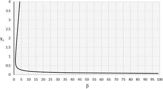
It is worth mentioning in this connection that Fig. 1 only partially covers the combination of discharge, water depth, channel width and side slope. For example for a trapezoidal channel with base width of 3 m and side slopes of 1 $H$ :0.5 $V$ on each side, a water depth of 3 meters will have a dimensionless depth $y_{u} =$ 3/(0.5*3)= 2 which cannot be read from Fig. 1 as the maximum dimensionless depth of flow available in the Fig. 1 is 1.0. For trapezoidal channels with narrower width and flatter slopes carrying water at greater depth, the dimensionless depth, $y_{2}$ can become large, much greater than one which limits the usage of dimensionless curves such as ones provided in Fig. 1. On the other hand, the proposed dimensionless curve provided in Fig. 7 can handle greater values of $y_{u}$ as high as four and simulate graphical determination of water depth at greater values of discharges.

For the circular shaped channels, the simulation of the graphical solution procedure was carried out with a dimensionless depth of flow varying between 0 and 1.0 and discharge values ranging between 0 and 4.0 m³/sec. It is to be noted that for circular shaped open channels, the maximum dimensionless depth of flow, $y_{u} (m a x)$ is 1.0 since $y_{u} = y / D$ and the depth of flow $y$ cannot exceed the dimeter, $D$ , of the circular shaped channel. Therefore, the maximum value of $y_{u} =$ 1.0 cannot be exceeded for circular shaped channels. Accordingly, the graphical plotting space prepared for circular shaped channels which is in accordance with Eq. (21) and is shown in Fig. 9 has a narrower range over which the specific energy function for circular shaped channels, $ϕ$ , varies compared to that of trapezoidal shaped channels. This range is given between $ϕ =$ 0 and $ϕ =$ 12 for the circular shaped channels as shown in Fig. 9.

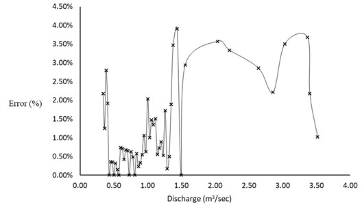
The results of the simulations for the graphical solution procedure are shown in Fig. 8 for trapezoidal shaped channels and Fig. 10 for the circular shaped channels. The graphs shows the plot of the percentage error in the determination of depth of flow over different values of discharge using the graphical solution implemented in accordance with the steps given above in Section 2.1.1 for trapezoidal shaped channels and Section 2.2.1 for circular shaped channels. It can be seen that the percentage error varies between 0 and 4 % for both shapes of channels. The mean percentage error of simulation is 1.13 % for trapezoidal shaped channels and 1.26 % for circular shaped channels. These percentage errors are small for a graphical solution procedure indicating the greater precision with which the proposed graphical solutions can be implemented for both the trapezoidal and circular shaped channels.

Fig. 8Variation of percentage error of relative depth determination with discharge in trapezoidal shaped channels from the graphical simulation

Variation of percentage error of relative depth determination with discharge in trapezoidal shaped channels from the graphical simulation

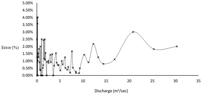
Fig. 9General graph used for simulation of depth determination in circular shaped channels with discharge ranging between 0-4 m3/sec

Examination of the percentage error graphs shown in Fig. 8 and Fig. 10 suggests that the percentage errors tend to grow higher at very small and very large values of discharges. The larger percentage of errors at smaller discharges can be explained by the fact that at smaller discharge values the dimensionless depth of flow is small. This will make the error from the graphical solution larger in comparison with the smaller dimensionless depth present in the flow. On the other side, the relatively greater percentage of errors present at large flows can be explained by the fact that the slope line, $η$ , for both the circular and trapezoidal shaped channels starts to coincide with the upper limbs of the dimensionless curves making it difficult to exactly locate the intersection point between the slope line and the dimensionless curves.

The determination of the dimensionless critical depth also requires careful alignment of the slope line until it becomes tangent to the dimensionless curve. This will be easier with better practice since the point at which the slope line becomes tangent to the curve will become apparent in the course of sliding the slop line over the curve in parallel motion whereby, as the line passes the tangent point, openings (gaps) start to appear slightly whereas the gaps are bigger at points away from the tangent point. This fact together with the zooming large capability available with graphical software programs such as Microsoft Excel can help in locating the tangent point with greater precision.

Further demonstration of the application of the proposed graphical solution for solving problems in open channel flows using specific energy is given below through application example for both trapezoidal and circular shaped channels.

Fig. 10Variation of percentage error of relative depth determination with discharge in circular shaped channels from the graphical simulation

Variation of percentage error of relative depth determination with discharge in circular shaped channels from the graphical simulation

5. Application examples

5.1. Example for trapezoidal channel

An example is given below for open channel flow in a trapezoidal shaped cross section having a base width of 3 m and side slopes of 1 horizontal to 0.5 vertical (Fig. 11). The flow in the channel is 5 m³/sec. The specific energy of flow in this channel is given as 1.0510 m. It is required to determine the alternate depths corresponding to this specific energy and the critical depth of flow.

Fig. 11Example for open channel flow in Trapezoidal shaped channel cross section

The graphical solution to this problem using the dimensionless graph is provided in Fig. 12. The procedure starts with computing the dimensionless quantities $θ^{3}$ and $η$ :

θ^{3} = \frac{Q^{2}}{g b^{5} m^{3}} = \frac{5^{2}}{9.81 * 3^{5} * 0 . 5^{3}} = 0.0838986,

η = \frac{Δ β}{(Δ y_{u})} = \frac{(θ^{3} - 1)}{θ^{3}} = \frac{(0.0839 - 1)}{0.0839} = - 10.91915 .

The dimensionless specific energy, $E_{u}$ is calculated as:

E_{u} = \frac{E}{m b} = \frac{1.0510}{0.5 * 3} = 0.700666 .

The $β$ -intercept is given by:

\frac{E_{u}}{θ^{3}} = \frac{0.700666}{0.083896} = 8.3513 .

Using the dimensionless curve shown in Fig. 12, the slope line, $η$ , is drawn by connecting $y_{u} =$ 1 on the vertical axis with $β =$ 10.92 on the horizontal axis. Next, sliding a line parallel to the $η$ -line and passing through the $β$ -intercept, i.e., $E_{u} / θ^{3} =$ 8.35 will produce the intersection points of the dimensionless curve with the parallel line. Drawing horizontal lines towards the vertical $y_{u}$ axis from these intersection points give the alternate dimensionless depths $y_{u 1}$ and $y_{u 2}$ . Accordingly, from Fig. 12:

y_{u 1} = 0.66, y_{u 2} = 0.24 .

The actual depths are:

y_{1} = y_{u 1} * m b = 0.66 * 0.5 * 3 = 0.99 m,

y_{1} = y_{u 2} * m b = 0.24 * 0.5 * 3 = 0.36 m .

The critical depth is likewise determined by sliding a line parallel to the $η$ -line until it touches the dimensionless $β$ - $y_{u}$ curve at tangent as shown in Fig. 12. This produces the dimensionless critical depth $y_{u c}$ of:

y_{u c} = 0.38 .

The actual critical depth is then calculated as:

y_{c} = y_{u c} * m b = 0.38 * 0.5 * 3 = 0.57 m .

Fig. 12Dimensionless Specific energy graph (β-yu) for trapezoidal channel

It is worthwhile to compare this graphical solution with numerical iterative procedures in order to appreciate how relatively easily the graphical solution has been obtained and the level of precision that can be attained with the graphical solution in comparison with the numerical procedures. Using the specific energy equation of Eq. (2) (with slight rearrangement) and substituting the given quantities will give:

E = 1.0510 = y + \frac{Q^{2}}{2 g y^{2} {(b + \frac{y}{m})}^{2}} = y + \frac{5^{2}}{2 * 9.81 y^{2} {(3 + 2 y)}^{2}} .

The above equation is rearranged into a five degree polynomial equation given below:

y^{5} + 1.949 y^{4} - 0.903 y^{3} - 2.36475 y^{2} + 0.31855 = 0 .

For a five degree polynomial equation, because of the impossibility of formulating analytical solution that can be traditionally expressed in radicals, an iterative numerical solution is a common alternative. Using polynomial solvers available on the internet, the following complete solutions are obtained:

y = \{0.3654, 1.0004, - 0.43465, - 1.17965, - 1.70015\} .

Therefore, the feasible solutions are given by:

y = \{0.3654 m, 1.004 m\} .

The graphical solution of $y =$ {0.36, 0.99} obtained earlier with relative ease is quite close to the numerical solution above with a maximum difference of about 1.5 %.

The graphical solution for the critical depth $y_{c}$ obtained earlier is likewise checked with the numerical solution as provided below. The critical depth is obtained by differentiating the specific energy with respect to the depth of flow and setting the result to zero:

E = y + \frac{v^{2}}{2 g} = y + \frac{Q^{2}}{2 g A^{2}},

\frac{d E}{d y} = 0 = 1 - \frac{Q^{2}}{g {A_{c}}^{3}} \frac{d A}{d y} = 1 - \frac{Q^{2} T_{c}}{g {A_{c}}^{3}} .

Rearranging gives:

\frac{Q^{2}}{g} = \frac{{A_{c}}^{3}}{T_{c}},

where $T$ is the top water surface width of the trapezoidal channel.

Substituting the given values of depth and discharge in the Application Example gives:

\frac{5^{2}}{9.81} = \frac{(3 y_{c} + 2 {y_{c}}^{2})^{3}}{(3 + 4 y_{c})} .

Rearranging the above equation further gives a six degree polynomial equation given below:

{y_{c}}^{6} + 4.5 {y_{c}}^{5} + 6.75 {y_{c}}^{4} + 3.375 {y_{c}}^{3} - 1.2792 y_{c} - 0.95566 = 0 .

Using again polynomial equation solver available over the internet, the solutions set of the above six degree equation is given as:

y_{c} = \{0.57398, - 0.877857, C o m p l e x n u m b e r s\} .

Accordingly, the feasible solution for the critical depth of flow is:

y_{c} = 0.574 m .

The graphical solution obtained earlier for the critical depth, $y_{c} =$ 0.57 compares quite well with the numerical solution above within two decimal places giving percentage difference of 0.7 %. In order to provide a comparison of the graphical solution obtained above with that of the earlier graphs, the problem is solved again using the dimensionless curves illustrated on the book by Jeppson [26], [27]. The solutions are shown in Fig. 13 for alternate depths determination and Fig. 14 for critical depth determination. It is seen that the latest publication of the book by Jeppson of 2011 improves the determination of the dimensionless critical depth for trapezoidal channels to just a single curve compared to the multiple curves provided by the earlier publication of 2010 each corresponding to specific values of side slope, $m$ .

According to the solution using the graphs of Fig. 13 for the alternate depths, a vertical line (shown in dotted red in Fig. 13) is drawn at the dimensionless specific energy value, $E_{u} =$ 0.7 that was worked out earlier in the illustration of the proposed graphical method. This vertical line should intersect the dimensionless curve corresponding to the value $Q'$ of:

Q' = \frac{Q^{2}}{g b^{5} m^{3}} = \frac{5^{2}}{9.81 * 3^{5} * 0 . 5^{3}} = 0.084 .

Since a curve corresponding to $Q' =$ 0.084 is not available in Fig. 13, interpolation shall be made between $Q^{'} =$ 0.08 and $Q' =$ 0.09. The corresponding values of $y_{u 1}$ and $y_{u 2}$ are 0.26 and 0.68. Accordingly the alternate depths will be $y_{1} =$ 0.26*0.5*3 = 0.39 m and $y_{2} =$ 0.68*0.5*3 = 1.02 m. Compared to the numerical solution of 0.3654 m and 1.004 m, these estimates have errors of 6.7 % and 1.6 % respectively. Apart from the relatively higher percentage errors made with the best of effort at interpolation, it should be noted that the higher value of the dimensionless depth is difficult to determine since the upper limbs of dimensionless curves are crowded and overlap with each other.

Fig. 13Solution to example for trapezoidal channel using the dimensionless curves from Jeppson [26]. The alternate depths in dimensionless forms are read horizontally from the intersection of the vertical redline with dimensionless curve interpolated for Q'= 0.083

Solution to example for trapezoidal channel using the dimensionless curves from Jeppson [26]. The alternate depths in dimensionless forms are read horizontally from the intersection of the vertical redline with dimensionless curve interpolated for Q'= 0.083

The critical depth is also estimated using the dimensionless curve provided by Jeppson and shown in Fig. 14. This improved version is better as it has only a single curve but has to be plotted separately from the curves given in Fig. 13 since the parameters of plot on the axis is now different. In Fig. 14 the $x$ -axis is plotted with $Q_{c}^{''} =$ 0.5* $Q^{'}$ . Again, a vertical line is drawn on Fig. 14 (show as dotted red line) corresponding to a $Q_{c}^{''}$ value of:

Q_{c}^{''} = \frac{Q^{2}}{2 g b^{5} m^{3}} = \frac{5^{2}}{289.81 * 3^{5} * 0 . 5^{3}} = 0.042 .

This vertical line intersects the $y_{c}^{'}$ curve at $y_{c}^{'}$ value of 0.4 which is read from the vertical $y_{c}^{'}$ axis by moving horizontally from the intersection between the vertical line and the $y_{c}^{'}$ curve. The critical depth is then calculated as $y_{c} =$ 0.4*0.5*3 = 0.6. Compared to the numerical value of 0.574 m worked out earlier this estimate represents an error or 4.5 % which is higher than the error produced by the application of the method proposed in this paper.

Fig. 14Critical flow conditions in trapezoidal channels, dimensionless graphs from Jeppson [29]. For the example problem of trapezoidal channels

Critical flow conditions in trapezoidal channels, dimensionless graphs from Jeppson [29]. For the example problem of trapezoidal channels

5.2. Example for a circular shaped channel

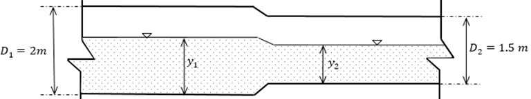
The example given below is taken from a book by R. Jeppson [26]. A transition occurs for an open channel flow of circular cross section shown in Fig. 15 from a 2 m diameter pipe to that of 1.5 m diameter. The transition keeps the centrelines of the two pipes lined up. For a flow rate of $Q =$ 2 m³/s, and a bottom slope of $S =$ 0.00095, and $n =$ 0.013, application of Manning’s Equation for the downstream section of 1.5 m diameter gave a normal depth $y_{2}$ of 1.131 m. For the upstream 2.0 m diameter pipe, it is required to determine the depth of flow y₁ just upstream from the transition. The solution so obtained is also to be verified by the numerical solution of the specific energy expressed in implicit form as given by Eq. (14).

Fig. 15Solved example: Circular shaped open channel transition from 2 m to 1.5 m diameter

The downstream dimensionless depth $y_{u 2}$ is given by:

y_{u 2} = \frac{y_{2}}{D_{2}} = \frac{1.131}{1.5} = 0.754 .

For the downstream 1.5 m diameter section, the dimensionless constants $α_{2}$ and the slope $η_{2}$ are determined as:

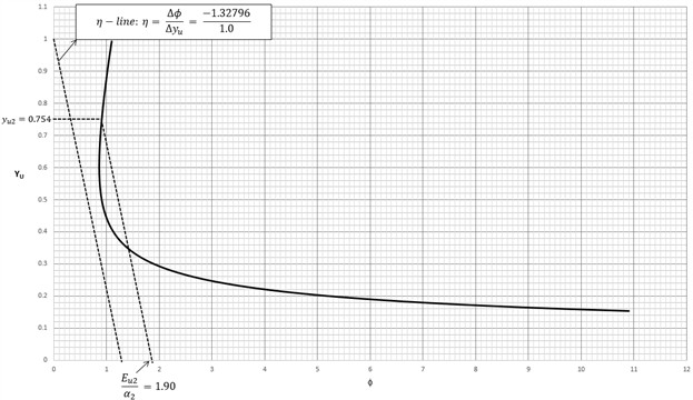
α_{2} = \frac{8 Q^{2}}{g D^{5}} = \frac{(8 * 2^{2})}{(9.81 * 1 . 5^{5})} = 0.42956,

η_{2} = \frac{Δ ϕ}{Δ y_{u}} = \frac{α_{2} - 1}{α_{2}} = \frac{0.42956 - 1}{0.42956} = - 1.32796 .

Using the dimensionless graph shown in Fig. 16, the slope line, $η_{2}$ , is drawn by connecting $y_{u} =$ 1 on the vertical axis with $ϕ =$ 1.32796 on the horizontal axis. Next, sliding a line parallel to the $η$ -line and passing through the dimensionless curve at $y_{u 2} =$ 0.754 will intersect the $ϕ$ axis at:

ϕ_{i 2} = \frac{E_{u 2}}{α_{2}} = 1.90 .

The dimensionless specific energy of the downstream 1.5 diameter section $E_{u 2}$ is then calculated as:

E_{u 2} = α_{2} (\frac{E_{u 2}}{α_{2}}) = 0.42956 * 1.90 = 0.81617 .

The specify energy $E_{2}$ of the downstream section is:

E_{2} = E_{u 2} D_{2} = 0.81617 * 1.5 = 1.22425 m .

To determine the Specific Energy of the upstream 2.0 m diameter channel section, Energy Equation is applied between the upstream and downstream sections of Fig. 15 and neglecting losses as follows:

E_{1} = y_{1} + \frac{{v_{1}}^{2}}{2 g} = 0.25 + y_{2} + \frac{{v_{2}}^{2}}{2 g} = 0.25 + E_{2},

E_{1} = 0.25 + E_{2} = 0.25 + 1.22425 = 1.4742 m .

The dimensionless specific energy is given by:

E_{u 1} = \frac{E_{1}}{D_{1}} = \frac{1.4742}{2.0} = 0.737124 .

For the upstream 2.0 m diameter section, the dimensionless constants $α_{1}$ and the slope $η_{1}$ are determined as:

α_{1} = \frac{8 Q^{2}}{g D^{5}} = \frac{(8 * 2^{2})}{(9.81 * 2 . 0^{5})} = 0.101937,

η_{1} = \frac{Δ ϕ}{Δ y_{u}} = \frac{α_{1} - 1}{α_{1}} = \frac{0.101937 - 1}{0.101937} = - 8.80998 .

The $ϕ$ -intercept is found from the formula:

ϕ_{i 1} = \frac{E_{u 1}}{α_{1}} = \frac{0.737124}{0.101937} = 7.2312 .

Using the dimensionless graph shown in Fig. 17, the slope line, $η_{1}$ , is drawn by connecting $y_{u} =$ 1 on the vertical axis with $ϕ =$ 8.81 on the horizontal axis. Next by sliding a line parallel to the $η_{1}$ -line and passing through the $ϕ$ - intercept, $ϕ_{i 1} =$ 7.23 will intersect the dimensionless $ϕ$ - $y_{u}$ curve $y_{u 1} =$ 0.725. The upstream depth of the 2.0 m diameter section just upstream of the transition is then given by:

y_{1} = y_{u 1} * D_{1} = 0.725 * 2.0 m = 1.45 m .

Fig. 16Example: Circular shaped channel. Using the dimensionless φ-yu curve to determine the ϕ-intercept, i.e., ϕi2=Eu2/α2 that gives the specific energy in the downstream 1.5 m diameter section of the channel

Example: Circular shaped channel. Using the dimensionless φ-yu curve to determine the ϕ-intercept, i.e., ϕi2=Eu2/α2 that gives the specific energy in the downstream 1.5 m diameter section of the channel

According to Jeppson [26] the numerical solution involving the implicit equation expressed either in terms of the depth $y_{1}$ or the angle $β$ using the Newton-Raphson method gives a solution for the upstream depth $y_{1} =$ 1.446. Therefore, the graphical method used in this example gives a result closer to the numerical solution with a margin of difference of 0.27 %.

For comparison purpose the example problem illustrated above is solved again using the curve provided by Jeppson and the graphical solution is shown in Fig. 18. Using the dimensionless depth $y_{u 2} =$ 0.754 computed above for the proposed method, a horizontal line is drawn from $y_{u} =$ 0.754 on the vertical axis of Fig. 18 until this horizontal line intersects the curve corresponding to the ${Q_{2}}^{'}$ value of:

25

Q_{2}^{'} = \frac{Q^{2}}{g {D_{2}}^{5}} = \frac{2^{2}}{(9.81 * 1 . 5^{5})} = 0.0537 .

Since dimensionless curve for $Q'$ is not available interpolation is made between $Q^{'} =$ 0.05 and $Q^{'} =$ 0.06. Drawing vertical line from this interpolated curve to the horizontal axis of the dimensionless specific energy gives $E_{u 2} =$ 0.8 shown with vertical dotted red line in Fig. 18. The corresponding downstream specific energy is $E_{2} =$ 0.8*1.5 = 1.2 m. Applying Energy equation between the downstream section 2 and upstream section 1 gives the upstream specific energy $E_{1}$ = 0.25+1.2 = 1.45 m. The dimensionless specific energy for the upstream section 1 is $E_{u 1} =$ 1.45/2 = 0.725. Drawing a vertical line on Fig. 18 (shown as blue dotted vertical line) at $E_{u} =$ 0.725 until this vertical line intersects the dimensionless curve corresponding to $Q_{1}^{'}$ value of:

Q_{1}^{'} = \frac{Q^{2}}{g {D_{1}}^{5}} = \frac{2^{2}}{(9.81 * 2 . 0^{5})} = 0.01274 .

Since a curve for $Q'$ is not available, interpolation is made between $Q^{'} =$ 0.01 and $Q^{'} =$ 0.02. Drawing a horizontal line from this interpolated curve on Fig. 18 until it intersects the vertical $y_{u}$ axis gives $y_{u 1} =$ 0.725. The upstream depth corresponding to this dimensionless depth is $y_{1} =$ 0.725*2 = 1.45. The value obtained is similar to the solution by the proposed graphical method which is somewhat a lucky outcome while interpolation had to be made twice for the dimensionless curves that are not available from Fig. 18. This can be a source of error that may affect the outcome.

Fig. 17Example: Circular shaped channel. Using the dimensionless ϕ-yu curve in which the upstream dimensionless depth yu1 of the 2.0 m diameter pipe section is determined by drawing the η-line through the ϕ-intercept, i.e., ϕi1=Eu1/α1=7.23 that intersects the dimensionless ϕ-yu curve at yu1= 0.725

Example: Circular shaped channel. Using the dimensionless ϕ-yu curve in which the upstream dimensionless depth yu1 of the 2.0 m diameter pipe section is determined by drawing the η-line through the ϕ-intercept, i.e., ϕi1=Eu1/α1=7.23 that intersects the dimensionless ϕ-yu curve at yu1= 0.725

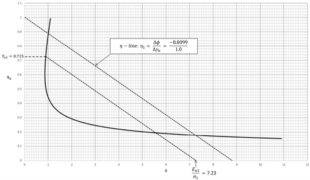
Fig. 18Solution to example problem of circular shaped channel using the dimensionless cure provided by Jeppson [26]. The red lines correspond to the downstream section 2 while the blue lines correspond to the upstream section 1

Solution to example problem of circular shaped channel using the dimensionless cure provided by Jeppson [26]. The red lines correspond to the downstream section 2 while the blue lines correspond to the upstream section 1

6. Discussion

Developing single, dimensionless specific energy curves for trapezoidal and circular shaped channels is difficult because of the existence of two independent dimensions in the equations even after dimensionless forms are formulated. These dimensions are the bottom width ( $b$ ) and side slopes ( $m$ ) for trapezoidal channels and the central angle ( $β$ ) defining depth of flow and the diameter ( $D$ ) for circular channels. In the past, the existence of such independent two dimensions in the dimensionless equations necessitated drawing discrete number of several curves that correspond to a combination of these dimensions. The method developed and presented in this paper systematically eliminated the existence of such dimensions and created an equation that is universally dimensionless for which a single curve can be drawn for each of the trapezoidal and circular channels. The methods developed above together with the application examples therefore show that it is possible to develop dimensionless graphs to analyse flow related problems which so far have not been possible for circular and trapezoidal shaped channels. The graphical procedure presented in this paper is simple to use requiring the definition of a slope of a line and $x$ -intercept after which a parallel line is drawn with the slope and the x-intercept so defined. The two intersection points between the slope line and the dimensionless curves gives the alternate depths of flow simultaneously. In addition, drawing the slope line at tangent to the dimensionless curves gives the critical depth flow, a depth that numerically necessitates solving a six degree polynomial equation for flows in trapezoidal shaped channels for which explicit algebraic solution form is not available.

Comparison of the graphical solution presented in this paper with the results obtained through numerical methods show that, with reasonably careful implementation of the graphical procedure, a good estimate that is close to the true depths can be obtained which for most practical purposes would be acceptable. By contrast, application of numerical methods requires either the use of trial and error procedure for solving polynomial equations of degree five or six for trapezoidal channels or transcendental equations for which explicit solutions are not available such as for flow in circular shaped cross sections. Adoption of numerical methods would often require the use of software programs for ease of implementation for all user environments. Comparison of the solution obtained for the example problems using the proposed graphical method with solutions obtained by graphical methods proposed such as the one used by Jeppson show that the proposed method has better accuracy with lower error margin of mostly less than 1 %. In addition the presence of just one universal dimensionless curve in the proposed method eliminates the confusion of locating intersection points where several dimensionless curves are crowded in overlapping manner as shown in Fig. 13 for trapezoidal channels and Fig. 18 for circular channels. In addition, the need for interpolating between the given dimensionless curves is avoided in the proposed which is not the case in the earlier graphs as the curves are drawn only for limited number of dimensionless parameter $Q'$ as shown in Fig. 13 and Fig. 18. Furthermore, the dimensionless curve for the determination of critical depth has to be drawn separately for both the trapezoidal as well as the circular cross sections. This requirement is avoided in the proposed graphical method because the same dimensionless curve is used for the determination of the critical depth as well as the alternate depths. This use of a single curve only is valid for both the trapezoidal and circular channel cross sections.

While numerical methods can be applied with a greater degree of accuracy, the argument that graphical methods are not forward looking is not entirely true and these methods can be applied in specific situations for design and analysis purposes. The dimensionless curves presented in this paper are universal and can be applied for any flow situation arising in trapezoidal and circular shaped channels. The procedures presented are simple and require the minimum of arithmetic operations and can be applied for estimating critical and alternate depths of flow. The example for the circular shaped channel shows that, where the specific energy along the channel is not the same because of changes in elevation of the bottom channel, simple application of energy equation enables the use of the dimensionless curve. Therefore, the dimensionless curves can be used for solving a wide variety of open channel flow problems involving specific energies which indicates the versatility of the use of such curves.

The proposed graphical procedure developed has an element of generality in that similar methods can be applied for graphically solving other hydraulic flow problems and not necessarily restricted to open channel flows only. Within the realm of open channel flows, one application example would be, for example solving normal depth problems in channels of different sections including trapezoidal, circular and other irregular shaped channels. Another example would be solving hydraulic problems in pressurized flows for example problems involving friction that are formulated based on the Colebrook-White equation for which the only graphical method available is the Moody Diagram that necessitates drawing several curves.

7. Conclusions

Open channel flow problems involving determination of alternate depth, critical depth and specific energy for trapezoidal and circular shaped channels require solving equations for which readymade explicit solutions are not available. Hydraulic engineering designs such as the design of stilling basins require determination of sequent depths and energy loss for which specific energy equation is useful [8]. In the case of trapezoidal and circular channels the solution of momentum and energy equations involve tedious trial and error procedures that are difficult to solve. Numerical solution procedures involving trial and error supported with linearization technique such as the Newton-Raphson method are commonly employed. Direct graphing is simple but is cumbersome and is only applicable to a specific flow problem. Semi-analytical solutions are available such as for circular channels but have limited range of applicability. Numerical techniques aimed at determining explicit solutions are widespread. However, such solutions, while possessing the power of great accuracy, can be quite complicated to formulate, understand and use. The use of dimensionless curves for circular and trapezoidal channels have in the past been formulated as a family of curves plotted for discrete combination of dimensionless variables and are not truly single universal curves. In such graphs, several of such curves have to be crowded into a plotting space. This paper demonstrated the development of a single universal dimensionless depth-specific energy curve for each of the trapezoidal and circular channels. It is shown further that such curves are simple to develop and use and provide accuracy that are reasonably comparable with numerical solutions. Simulation of the graphical solution over broader range of flows and dimensionless depth of flow shows that the solution is reasonably accurate with percentage error of estimation of depth varying between 0 and 4 % with mean percentage error of 1.1 % for trapezoidal shaped channels and 1.2 % for circular shaped channels. The use of these dimensionless curves can be adapted to wide range of user environments with inherent simplicity in their use. There is also a hint of a possibility in future of using similar procedure for solving other types of open channel flow related problems graphically. An example in which the proposed graphical method can be applied could be determining the required alternate depths of flow of a hydraulic jump used in stilling basin design in order to achieve a given percentage of energy loss. Channel cross sections such triangular and trapezoidal sections can be suitably handled using this proposed graphical method thereby eliminating the need for numerical iterative procedures normally employed in such channel cross sections. The proposed graphical method can also be applied in designing channel cross sections approaching control sections such as in inverted siphons where adequate depth of flow in the upstream approach channel must be provided particularly during low flow periods to avoid surface water level draw down that can create air entrainment inside inverted siphon pipe section. Further application of the proposed graphical method could be the design of open channels cross sections upstream of a control section where the flow passes through critical depth in which the upstream normal depth should be large enough to avoid chocking condition and erosion of the channel.

References

A. R. Vatankhah, “Explicit solutions for critical and normal depths in trapezoidal and parabolic open channels,” Ain Shams Engineering Journal, Vol. 4, No. 1, pp. 17–23, Mar. 2013, https://doi.org/10.1016/j.asej.2012.05.002

Publisher
T. Cheng, J. Wang, and J. Sui, “Calculation of critical flow depth using method of algebraic inequality,” Journal of Hydrology and Hydromechanics, Vol. 66, No. 3, pp. 316–322, Sep. 2018, https://doi.org/10.2478/johh-2018-0020

Publisher
H. Shang, S. Xu, K. Zhang, and L. Zhao, “Explicit solution for critical depth in closed conduits flowing partly full,” Water, Vol. 11, No. 10, p. 2124, Oct. 2019, https://doi.org/10.3390/w11102124

Publisher
Z. Z. Wang, T. Chen, X. M. Zhang, and X. D. Zhang, “Approximate solution for the critical depth of an arched tunnel,” Journal of Tsinghua University (Science and Technology), Vol. 44, pp. 812–814, 2004.

Search CrossRef
R. V. Raikar, M. S. Shiva Reddy, and G. K. Vishwanadh, “Normal and critical depth computations for egg-shaped conduit sections,” Flow Measurement and Instrumentation, Vol. 21, No. 3, pp. 367–372, Sep. 2010, https://doi.org/10.1016/j.flowmeasinst.2010.04.007

Publisher
A. R. Vatankhah, “Limiting dimensions for trapezoidal channels and control notches (Design Aid),” KSCE Journal of Civil Engineering, Vol. 17, No. 4, pp. 850–857, May 2013, https://doi.org/10.1007/s12205-013-0186-3

Publisher
H. Arvanaghi, G. Mahtabi, and M. Rashidi, “New solutions for estimation of critical depth in trapezoidal cross section,” Journal of Materials and Environmental Science, Vol. 6, No. 9, pp. 2453–2460, 2015.

Search CrossRef
Rashwan and I. M. H., “Analytical solution to problems of hydraulic jump in horizontal triangular channels,” Ain Shams Engineering Journal, Vol. 4, No. 3, pp. 365–368, Sep. 2013, https://doi.org/10.1016/j.asej.2012.11.007

Publisher
A. Das, “Solution of specific energy and specific force equations,” Journal of Irrigation and Drainage Engineering, Vol. 133, No. 4, pp. 407–410, Aug. 2007, https://doi.org/10.1061/(asce)0733-9437(2007)133:4(407)

Publisher
P. K. Swamee and P. N. Rathie, “Exact solutions for normal depth problem,” Journal of Hydraulic Research, Vol. 42, No. 5, pp. 543–550, Dec. 2010, https://doi.org/10.1080/00221686.2004.9641223

Publisher
P. K. Swamee and P. N. Rathie, “Exact equations for critical depth in a trapezoidal canal,” Journal of Irrigation and Drainage Engineering, Vol. 131, No. 5, pp. 474–476, Oct. 2005, https://doi.org/10.1061/(asce)0733-9437(2005)131:5(474)

Publisher
A. R. Vatankhah and S. Kouchakzadeh, “Discussion of Exact equations for critical depth in trapezoidal canal,” Journal of Irrigation and Drainage Engineering ASCE, Vol. 133, No. 5, pp. 508–508, May 2007.

Publisher
T. S. W. Wong and M. C. Zhou, “Determination of critical and normal depths using Excel,” in World Water and Environmental Resources Congress 2004, pp. 1–8, Jun. 2004, https://doi.org/10.1061/40737(2004)191

Publisher
A. Kanani, M. Bakhtiari, S. M. Borghei, and D.-S. Jeng, “Evolutionary algorithms for the determination of critical depths in conduits,” Journal of Irrigation and Drainage Engineering, Vol. 134, No. 6, pp. 847–852, Dec. 2008, https://doi.org/10.1061/(asce)0733-9437(2008)134:6(847)

Publisher
A. K. Mohammed, R. H. Irzooki, A. A. Jamel, W. S. Mohammed-Ali, and S. S. Abbas, “Novel approach to computing critical and normal depth in circular channels,” Mathematical Modelling of Engineering Problems, Vol. 8, No. 6, pp. 923–927, Dec. 2021, https://doi.org/10.18280/mmep.080611

Publisher
Z. Wang, “Formula for calculating critical depth of trapezoidal open channel,” Journal of Hydraulic Engineering, Vol. 124, No. 1, p. 90, Jan. 1998, https://doi.org/10.1061/(asce)0733-9429(1998)124:1(90)

Publisher
V. Ferro and M. Sciacca, “Explicit equations for uniform flow depth,” Journal of Irrigation and Drainage Engineering, Vol. 143, No. 5, pp. 1239–1246, May 2017, https://doi.org/10.1061/(asce)ir.1943-4774.0001152

Publisher
W. Straub, “A quick and easy way to calculate critical and conjugate depths in circular open channels,” Journal of Civil Engineering, pp. 70–71, 1978.

Search CrossRef
V. Chow, Open Channel Hydraulics. New York, N.Y: McGraw-Hill Book Co. Inc., 1958.

Search CrossRef
R. French, Open Channel Hydraulics. New York, N.Y.: McGraw-Hill Book Co. Inc., 1987.

Search CrossRef
F. Henderson, Open Channel Flow. New York, N.Y.: Macmillan Company, 1966.

Search CrossRef
K. Babaeyan-Koopaei, “Dimensionless curves for normal-depth calculations in canal sections,” Journal of Irrigation and Drainage Engineering, Vol. 127, No. 6, pp. 386–389, Dec. 2001, https://doi.org/10.1061/(asce)0733-9437(2001)127:6(386)

Publisher
M. Kc, J. Devkota, and X. Fang, “Comprehensive evaluation and new development of determination of critical and normal depths for different types of open-channel cross-sections,” in World Environmental and Water Resources Congress 2010, pp. 2058–2068, May 2010, https://doi.org/10.1061/41114(371)214

Publisher
M. B. Sonnen, “Discussion of “Dimensionless curves for normal-depth calculations in canal sections” by K. Babaeyan-Koopaei,” Journal of Irrigation and Drainage Engineering, Vol. 129, No. 3, pp. 223–224, Jun. 2003, https://doi.org/10.1061/(asce)0733-9437(2003)129:3(223)

Publisher
“Design of small canal structures,” U.S. Government Printing Office, Washington, D.C, USBR, 1978.

Search CrossRef
R. Jeppson, “Open Channel flows: Numerical methods and computer applications,” Taylor and Francis Group, 6000 Broken Sound Parkway NW, Suite 300, 2010.

Search CrossRef
B. Achour and M. Khattaoui, “Computation of normal and critical depths in parabolic cross sections,” The Open Civil Engineering Journal, Vol. 2, No. 1, pp. 9–14, Mar. 2008, https://doi.org/10.2174/1874149500802010009

Publisher

About this article

Received

February 24, 2025

Accepted

August 27, 2025

Published

September 29, 2025

DOI

https://doi.org/10.21595/mme.2025.24850

Keywords

open channel flow

specific energy

critical depth

dimensionless graphs

trapezoidal channels

circular channels

alternate depths

Data Availability

The datasets generated during and/or analyzed during the current study are available from the corresponding author on reasonable request.

Conflict of interest

The authors declare that they have no conflict of interest.

This is an open access article distributed under the Creative Commons Attribution License, which permits unrestricted use, distribution, and reproduction in any medium, provided the original work is properly cited.

Next article in issue Next

A. T. Tiruneh, “Single universal dimensionless specific energy curves for trapezoidal and circular shaped open channels,” Mathematical Models in Engineering, Vol. 11, No. 3, pp. 68–96, Sep. 2025, https://doi.org/10.21595/mme.2025.24850

Copy Extrica

Copied to clipboard!

TY  - JOUR
DO  - 10.21595/mme.2025.24850
UR  - https://doi.org/10.21595/mme.2025.24850
TI  - Single universal dimensionless specific energy curves for trapezoidal and circular shaped open channels
T2  - Mathematical Models in Engineering
AU  - Tiruneh, Ababu T.
PY  - 2025
DA  - 2025/09/29
PB  - Extrica
SP  - 68-96
VL  - 11
IS  - 3
SN  - 2351-5279
SN  - 2424-4627
ER  - 

Copy Ris

Copied to clipboard!

 @article{Tiruneh_2025, title={Single universal dimensionless specific energy curves for trapezoidal and circular shaped open channels}, volume={11}, ISSN={2424-4627}, url={https://doi.org/10.21595/mme.2025.24850}, DOI={10.21595/mme.2025.24850}, number={3}, journal={Mathematical Models in Engineering}, publisher={JVE International Ltd.}, author={Tiruneh, Ababu T.}, year={2025}, month=sep, pages={68–96} }

Copy Bibtex

Copied to clipboard!

[1]A. T. Tiruneh, “Single universal dimensionless specific energy curves for trapezoidal and circular shaped open channels,” Mathematical Models in Engineering, vol. 11, no. 3, pp. 68–96, Sep. 2025, doi: 10.21595/mme.2025.24850.

Copy IEEE

Copied to clipboard!

Tiruneh, Ababu T. “Single Universal Dimensionless Specific Energy Curves for Trapezoidal and Circular Shaped Open Channels.” Mathematical Models in Engineering 11, no. 3 (September 29, 2025): 68–96. https://doi.org/10.21595/mme.2025.24850.

Copy Chicago

Copied to clipboard!

Single universal dimensionless specific energy curves for trapezoidal and circular shaped open channels

Abstract

Highlights

1. Introduction

2. Objective of the proposed graphical method

3. Methods

3.1. Trapezoidal channels

3.2. Procedure for developing and using the universal dimensionless specific energy curve for trapezoidal channel cross sections.

3.3. Circular channels

3.4. Procedure for developing and using the universal dimensionless specific energy curve for trapezoidal channel cross sections

4. Results

5. Application examples

5.1. Example for trapezoidal channel

5.2. Example for a circular shaped channel

6. Discussion

7. Conclusions

References

About this article

Related Articles