A bearing fault diagnosis method based on MCDCGAN and DPTAN under data imbalance

Zhang, Sen; Yan, Le; Liu, Zhaodong; Ren, Hao; Lu, Heng

doi:10.21595/jme.2026.25374

Journal of Measurements in Engineering

Browse Journal

Submit article

Published: August 3, 2026

Check for updates

A bearing fault diagnosis method based on MCDCGAN and DPTAN under data imbalance

Sen Zhang¹

Le Yan²

Zhaodong Liu³

Hao Ren⁴

Heng Lu⁵

^{1, 2, 3}School of Automation and Electrical Engineering, Linyi University, Linyi, 276000, China

⁴School of Information Science and Engineering, East China University of Science and Technology, Shanghai 200237, China

⁵Department of Information Engineering, Linyi Vocational University of Science and Technology, Linyi, 276025, China

Corresponding Authors:

Zhaodong Liu, Heng Lu

Cite the article Download PDF

Article in Press

Downloads 0

Abstract

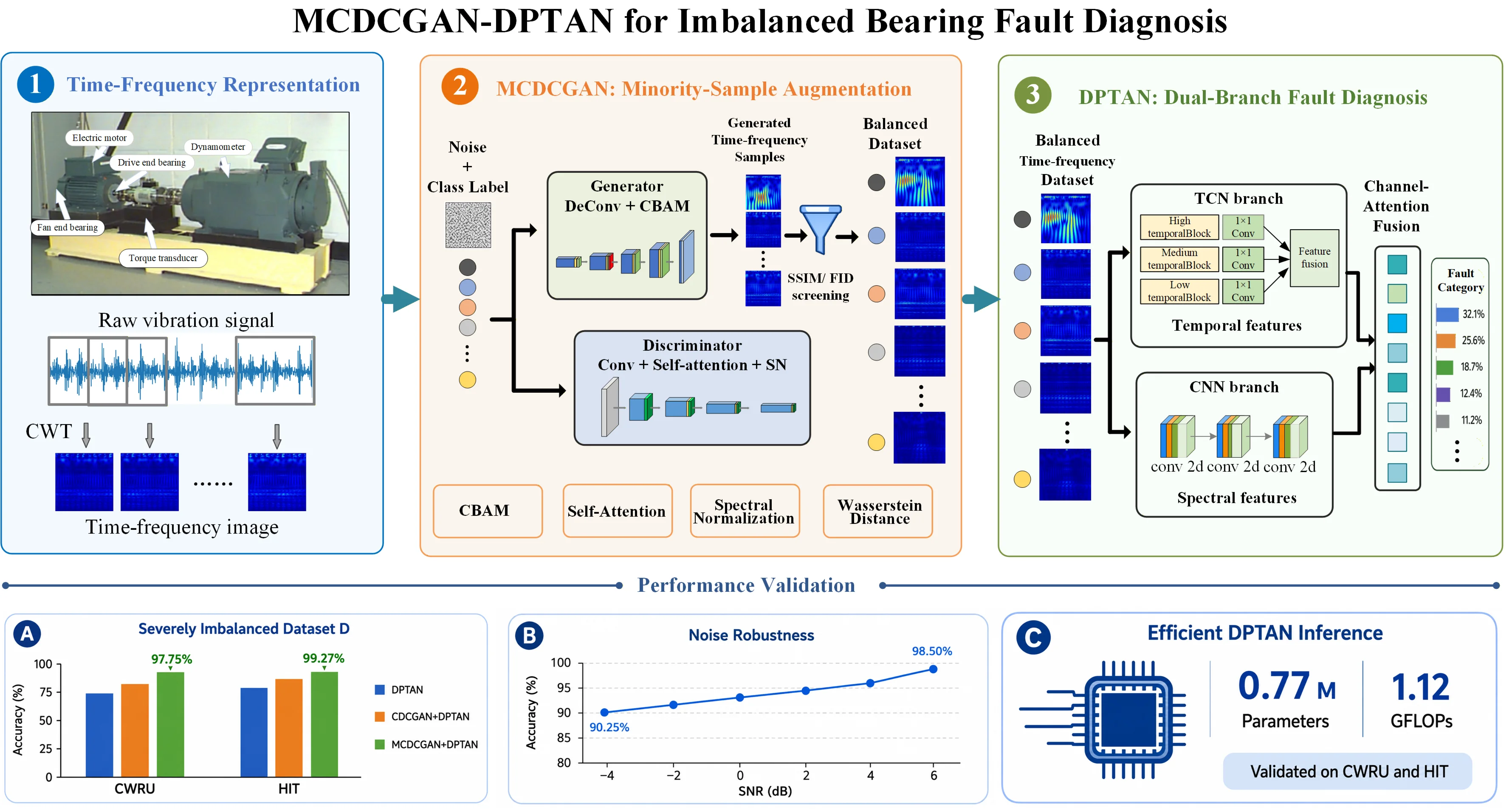
Bearings are critical components of rotating machinery, yet reliable fault diagnosis remains challenging under complex conditions due to signal non-stationarity and data scarcity. To address these issues, this paper proposes a diagnostic framework that combines generative-adversarial data augmentation with dual-branch time–frequency representation learning to improve feature quality and fault classification. Firstly, the bearing vibration signals are transformed into two-dimensional time-frequency representations by utilizing the continuous wavelet transform. Subsequently, a multi-attention conditional deep convolutional generative adversarial network (MCDCGAN) is employed for conditional augmentation under class imbalance, integrating attention mechanisms and stabilization strategies to generate more reliable samples for minority fault classes. Finally, a dual-branch parallel time-frequency attention network (DPTAN) is designed to jointly learn temporal and spectral feature representations and then fuse them for fault classification. Experimental results on the CWRU and HIT datasets demonstrate that the proposed method achieves better performance than baseline models and maintains robustness under data imbalance and noisy conditions.

A bearing fault diagnosis method based on MCDCGAN and DPTAN under data imbalance

Highlights

MCDCGAN improves minority-class sample quality under severe data imbalance.
DPTAN jointly learns temporal and spectral features with attention-based fusion.
The framework achieves robust diagnosis on both CWRU and HIT bearing datasets.

1. Introduction

The increasing complexity of modern mechanical systems, driven by rapid advancement of intelligent manufacturing and industrialization, presents significant challenges to reliable fault diagnosis [1], [2]. Rolling bearings are critical components in rotating machinery and one of the main fault sources in industrial systems. The conventional fault diagnosis methods extract fault features from the original vibration signals by using signal processing techniques, and then identify and classify the potential faults [3]. These methods rely heavily on domain expertise and sophisticated signal processing capabilities [4].

As a mainstream approach in fault diagnosis, deep learning not only extracts and classifies bearing fault features, but also reduces reliance on expert knowledge while improving diagnosis accuracy [5], [6]. Early deep learning approaches, including convolutional neural networks (CNN) and recurrent neural networks (RNN), have achieved successful applications. For instance, a mixed data input bearing fault diagnosis method was proposed to locate bearing faults, achieving high diagnostic accuracy [7]. In [8], the gramian angular field transformation, extreme learning machine and CNN were combined to classify various fault types with strong generalization ability. Based on the integration of CNN and attention mechanisms, a diagnostic scheme was proposed in [9] to optimize the accuracy of bearing fault identification.

In recent years, the deep learning field has witnessed a significant paradigm shift towards more sophisticated architectures, with the most notably being transformers and diffusion models. Transformers, leveraging self-attention modules, are adept at learning long-range relationships in signal data. For example, Wang et al. [10] provided a comprehensive survey on transformer-based intelligent fault diagnosis, highlighting their superiority in modeling complex temporal relationships. Similarly, diffusion models have emerged as a powerful tool for high-quality sample generation and anomaly detection [11]. Alongside these architectural advances, multi-sensor fusion and attention mechanisms have attracted considerable research interest in enhancing feature extraction in complex operating environments. Ye et al. [12] proposed a multi-sensor residual convolutional fusion network to effectively fuse multi-source information. Yan et al. [13] developed a coarse-to-fine dual-scale time-frequency attention fusion network for compound fault diagnosis. Furthermore, for the sake of addressing variable working conditions, a multi-branch attention coupled convolutional domain adaptation network was introduced in [14]. Other notable works include the multi-sensor information fusion deep ensemble learning network [15] and advanced methods for remaining useful life prediction [16]. These state-of-the-art studies demonstrate that integrating attention mechanisms and advanced fusion strategies is a promising direction for improving diagnostic performance.

Despite these advancements, practical applications still face the challenge of serious imbalance in sample distribution, where the number of normal samples far exceeds that of fault samples. Unbalanced sample distribution often leads to biased model training, which reduces the performance of fault classification [17], [18]. Traditional resampling and cost-sensitive learning methods have limited effect in solving the problem of unbalanced sample distribution, and these methods may inject artificial noises, discard informative samples, or rely on unrealistic cost assumptions [19]. The generative adversarial networks (GANs) can generate minority samples and balance the sample distribution without damaging the majority samples. The first-ever GAN was proposed in [20], and since then, GANs have been a hot topic of research that stirs considerable interest in the machine learning community. By integrating deep convolutional neural networks and conditional GANs, reference [21] designed an improved conditional deep convolutional generative adversarial network (CDCGAN) for supporting the training of the CNN-SVM diagnostic model. The enhanced GAN model incorporating attention mechanisms and global feature crossover was considered in [22] for improving feature learning and noises robustness capabilities under limited data conditions. In [23], an auxiliary classifier generative adversarial network (ACGAN) was enhanced by integrating Wasserstein distance and multi-level attention to boost the quality of synthetic samples. While diffusion models are gaining traction, GANs remain highly efficient for real-time sample generation in industrial scenarios.

It is worth noting that feature extraction is crucial for bearing fault diagnosis, which directly determines whether the model can identify the relevant fault information from the original signals [24]. Most existing feature extraction methods generally adopt a single network architecture, such as CNN or temporal convolutional network (TCN), which limits the utilization of complementary time-frequency information. For example, a lightweight CNN architecture was designed in [25] through neural architecture search and network pruning. In [26], the self-attention mechanism combining TCN and the soft threshold algorithm was developed for intelligent fault identification. Based on signal-to-image transformation and CNN, a novel fault classification framework was proposed in [27] to achieve automatic identification of bearing faults. In addition, the fast Fourier transform and attention mechanism were introduced in the TCN to achieve deep fault feature extraction in [28]. Following this line, and inspired by the recent success of fusion and attention networks [12-15], a natural idea is to combine TCN and CNN with advanced attention mechanisms to improve the competence of bearing feature extraction.

In response to the aforementioned motivations, this paper proposes a novel bearing fault diagnosis method based on a multi-attention conditional deep convolutional generative adversarial network (MCDCGAN) and a dual-branch parallel time-frequency attention network (DPTAN). The main contributions of this paper can be highlighted as follows.

1) Under the condition of unbalanced bearing data, this paper proposes a bearing fault diagnosis method based on MCDCGAN and DPTAN.

2) Considering the unbalanced distribution of fault data, an augmentation model MCDCGAN is developed by combining the Wasserstein distance, spectral normalization, self-attention mechanism and convolution block attention module (CBAM).

3) Based on CNN and TCN, a DPTAN is designed for improving the performance of bearing fault classification.

The subsequent sections are structured as follows. Section 2 introduces the relevant theoretical foundations, including continuous wavelet transform (CWT), CDCGAN, Wasserstein distance, spectral normalization, and attention mechanisms. Section 3 elaborates on the proposed MCDCGAN model and DPTAN model. In Section 4, experimental verification and discussions are conducted to demonstrate the effectiveness of the proposed methods. Finally, Section 5 concludes the article.

2. Related theories

2.1. CWT theory

Industrial bearing systems often operate under non-stationary conditions, and traditional methods based on frequency or time domain cannot accurately capture the transient fault characteristics, which makes bearing fault diagnosis extremely difficult. The CWT performs localized time-frequency analysis by calculating the inner product between the input signal and a series of wavelet functions at various scales and positions [29], [30]. Different from the Fourier transform, CWT is more suitable for processing non-stationary signals and can record instantaneous features at various time scales. The mathematical formulation of CWT is presented as follows:

1

W (a, b) = \frac{1}{\sqrt{a}} \int_{- \infty}^{\infty} x_{t} φ^{*} (\frac{t - b}{a}) d t,

where $x_{t}$ denotes the input signal, $φ^{*} (\cdot)$ represents the mother wavelet, $a$ and $b$ are continuous parameters that control the scaling and translation of the wavelet, respectively.

2.2. CDCGAN theory

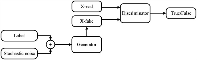
The original GAN constructs the network according to the fully connected layer. In contrast, DCGAN replaces the fully connected layer to the convolutional layer, which significantly improves the feature extraction capability. CDCGAN is an improved model based on DCGAN, which can achieve the control of the generated samples by introducing conditional information [31], [32]. The model generator produces the specified samples X-fake based on the label information. Then, the generated samples X-fake and the real samples X-real are alternately input into the discriminator to train the ability to discriminate the generated samples and the real samples. The structure of CDCGAN is shown in Fig. 1.

Fig. 1The structure of CDCGAN

2.3. GAN improvement strategy

2.3.1. Wasserstein distance

The Wasserstein distance can effectively quantify the distribution difference between the generated samples and the real samples and is widely adopted as a loss function in the generation models [33], [34]. Besides, the continuity of the Wasserstein distance provides a smooth and non-zero gradient signal, which significantly improves the training stability of the GAN. The following is the description of Wasserstein distance:

2

W (P_{d a t a}, P_{g}) = \underset{γ \in Γ (P_{d a t a}, P_{g})}{i n f} E_{(x, y) \sim γ} [∥ x - y ∥],

where $Γ (P_{d a t a}, P_{g})$ represents the set of all possible joint distributions for the combination $P_{d a t a}$ and $P_{g}$ , and $E_{(x, y) \sim γ} [∥ x - y ∥]$ is the expectation of the samples under $γ$ with respect to the distance.

2.3.2. Spectral normalization

In order to satisfy the 1-Lipschitz condition of the Wasserstein distance, the original Wasserstein GAN applies weight clipping to the discriminator parameters. However, weight clipping would excessively constrain the parameter space of the discriminator, resulting in limited function expression ability and reducing the effectiveness of adversarial training. The spectral normalization constrains the weight matrix in each layer based on the maximum singular value [35], which can ensure the excellent expressive capability of the model while satisfying the Lipschitz constraint. For a weight matrix $W$ , the spectral normalization is defined as:

3

\tilde{W} = \frac{W}{σ (W)},

where $σ (W)$ denotes the largest singular value of $W$ .

2.3.3. Attention mechanisms

The attention mechanism improves the learning capability of fault feature representation by guiding a model to dynamically concentrate on the information that is most relevant to the current fault diagnosis process. According to [36], the CBAM integrates the spatial attention module (SAM) and the channel attention module (CAM), which can enhance the feature representation. The overall structure is shown in Fig. 2.

Fig. 2The structure of CBAM

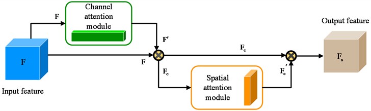
In particular, CAM adaptively adjusts the weights of different channels to highlight discriminative channel information, and SAM enables the model to selectively attend to spatial regions that contribute most to the fault diagnosis task. The self-attention mechanism establishes a global feature association through the pairwise similarity calculation between features, which can effectively capture the dependence of long-term distance. This mechanism can dynamically adjust the interaction weights between features, so that the model has stronger expression ability when dealing with multi-scale features or non-local information.

3. Methodology

In this paper, the proposed bearing fault diagnosis method includes two main functional modules, namely MCDCGAN data augmentation module and DPTAN fault classification module. As illustrated in Fig. 3, the method consists of three consecutive stages.

Fig. 3The flowchart of proposed method

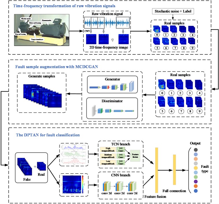
Phase 1: Time-frequency transformation of raw vibration signals. In the data preprocessing part, this paper first divides the raw vibration signals into signal segments by using the sliding window overlapping sampling strategy. After that, the intercepted signal segments are converted into two-dimensional time-frequency representations by CWT.

Phase 2: Fault sample augmentation with MCDCGAN. The MCDCGAN model is designed to enhance the two-dimensional time-frequency representations of fault samples. By generating high-quality synthetic samples to supplement the original dataset, an augmented dataset with balanced category distribution is constructed for subsequent fault diagnosis tasks.

Phase 3: The DPTAN for fault classification. The augmented dataset is input into the DPTAN model for fault classification. The model adopts a dual-branch architecture: the temporal branch employs TCN to extract temporal features and the frequency branch utilizes CNN to extract spectral features. Based on the attention mechanism, the temporal and frequency domain features are adaptively fused, ultimately outputting the probability distribution of fault categories.

3.1. MCDCGAN module

The Fig. 4 illustrates the structure of MCDCGAN, which consists of a generator and a discriminator. The generator adopts a dual-branch input architecture to process stochastic noises and conditional category labels respectively. In addition, the generator employs a five-layer transposed convolutional network to achieve progressive spatial upsampling, and each layer is equipped with batch normalization followed by a ReLU nonlinearity. Moreover, the CBAM attention module is integrated into the specific intermediate feature layers to enhance the feature selection capacity. Finally, the output is mapped to the standardized range according to the Tanh activation function. On the other hand, the discriminator also employs a dual-branch input architecture to process time-frequency images and conditional category labels respectively. Besides, the discriminator achieves feature extraction and image authenticity discrimination based on a five-layer convolutional network, where each layer applies spectral normalization and the LeakyReLU activation function to ensure training stability. Finally, the discriminator integrates a self-attention module in the key intermediate feature layer to capture long-range spatial correlations.

Fig. 4The structure of MCDCGAN

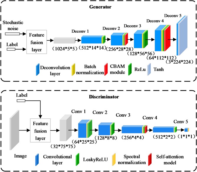
In this study, a multi-attention optimization strategy is integrated into the MCDCGAN model to strengthen the quality of synthesized fault samples. In the generator, the CBAM module is deployed at the second and fourth transposed convolutional layers, and the spatial resolution and semantic representation capabilities of these layers are further utilized to achieve dynamic feature weighting, thereby enhancing the perception of key information regions and suppressing redundant information interference. In the discriminator, the self-attention module is located after the third convolutional layer, and the query-key-value fusion spectral normalization architecture is adopted to capture the long-range spatial correlation by calculating the spatial attention weight matrix, thereby improving the accuracy of true and false sample discrimination. In short, this dual attention design can accurately perceive global structural features and extract key features, significantly improving image generation quality, diversity and training stability.

In this paper, a loss function based on the Wasserstein distance is employed in MCDCGAN. The Wasserstein distance constructs a smoother and more informative objective function, which ensures effective gradient propagation and model optimization. In the MCDCGAN, the loss function is defined as:

4

\{\begin{array}{l} L_{D} = - (m e a n (y_{r e a l}) - m e a n (y_{f a k e})), \\ L_{G} = - m e a n (y_{f a k e}), \end{array}

where $y_{r e a l}$ represents the predictive output of the discriminator for the real samples and $y_{f a k e}$ represents the predictive output of the discriminator for the generated samples.

In order to ensure the training stability and convergence of the MCDCGAN model, the key hyperparameters are carefully configured in this study. In terms of learning rate setting, the generator and discriminator adopt the differentiation strategy of 0.0001 and 0.0003 respectively, and provide more accurate gradient guidance for the generator by improving the learning speed of the discriminator. A batch size of 16 is adopted, which strikes a trade-off between computational efficiency and training stability. The generator and discriminator use convolution kernels of 4×4 and 5×5, respectively. Table 1 lists the complete parameters configuration of MCDCGAN.

Table 1The parameters of MCDCGAN

Generator	Parameters	Discriminator	Parameters
Input noise	$x \in R^{100 \times 1 \times 1}$	Input image	$x \in R^{3 \times 224 \times 224}$
Input label	$y \in R^{10 \times 1 \times 1}$	Input label	$y \in R^{10 \times 224 \times 224}$
DeConv_x	in: 100, out: 512, $k =$ 5, $s =$ 1, $p =$ 0, BN = 512, Act: ReLU	Conv_x	in: 3, out: 16, $k =$ 5, $s =$ 3, $p =$ 3, SN, Act: LReLU
DeConv_y	in: 10, out: 512, $k =$ 5, $s =$ 1, $p =$ 0, BN = 512, Act: ReLU	Conv_y	in: 10, out: 16, $k =$ 5, $s =$ 3, $p =$ 3, SN, Act: LReLU
Concat	$c =$ 1024, $h =$ 5, $w =$ 5	Concat	$c =$ 32, $h =$ 75, $w =$ 75
DeConv1	in: 1024, out: 512, $k =$ 4, $s =$ 3, $p =$ 1, BN = 512, Act: ReLU	Conv1	in: 32, out: 64, $k =$ 5, $s =$ 3, $p =$ 2, SN, Act: LReLU
DeConv2	in: 512, out: 256, k = 4, s = 2, $p =$ 1, BN = 256, Act: ReLU	Conv2	in: 64, out: 128, $k =$ 5, $s =$ 3, $p =$ 0, SN, Act: LReLU
Channel attention	in: 256, ratio = 16, Act: Sigmoid	Conv3	in: 128, out: 256, $k =$ 5, $s =$ 3, $p =$ 3, SN, Act: LReLU
Spatial attention	kernel = 7, padding = 3, Act: Sigmoid	Query conv	in: 256, out: 64, $k =$ 1, SN
DeConv3	in: 256, out: 128, $k =$ 4, $s =$ 2, $p =$ 1, BN = 128, Act: ReLU	Key conv	in: 256, out: 64, $k =$ 1, SN
DeConv4	in: 128, out: 64, $k =$ 4, $s =$ 2, $p =$ 1, BN = 64, Act: ReLU	Value conv	in: 256, out: 256, $k =$ 1, SN
Channel attention	in: 64, ratio = 16, Act: Sigmoid	Conv4	in: 256, out: 512, $k =$ 5, $s =$ 3, $p =$ 2, SN, Act: LReLU
Spatial attention	kernel = 7, padding = 3, Act: Sigmoid	Conv5	in: 512, out: 1, $k =$ 4, $s =$ 2, $p =$ 1, SN, Act: LReLU
DeConv5	in: 64, out: 3, $k =$ 4, $s =$ 2, $p =$ 1, Act: Tanh

The model is trained for 200 epochs, and the optimal performance model is dynamically saved based on structural similarity index measure (SSIM) and Fréchet inception distance (FID) indicators during the training process. After the training is completed, the proposed method in this paper generates fault samples according to the best model, and establishes an automatic image quality screening mechanism based on SSIM and FID. The relevant indicators are as follows:

5

\{\begin{array}{l} S S I M (x, y) = \frac{(2 μ_{x} μ_{y} + a_{1}) (2 σ_{x y} + a_{2})}{(μ_{x}^{2} + μ_{y}^{2} + a_{1}) (σ_{x}^{2} + σ_{y}^{2} + a_{2})} \geq 0.6, \\ F I D = | | μ_{r} - μ_{g} | |^{2} + T r (Σ_{r} + Σ_{g} - 2 (Σ_{r} Σ_{g})^{\frac{1}{2}}) \leq 180, \end{array}

where $μ_{x}$ , $μ_{y}$ , $σ_{x}$ , $σ_{y}$ , and $σ_{x y}$ denote the mean, standard deviation and covariance of pixel intensities of images $x$ and $y$ , respectively. $a_{1}$ and $a_{2}$ are constants. The means and covariance matrices of generated and real image features are indicated by $μ_{r}$ , $μ_{g}$ , $Σ_{r}$ and $Σ_{g}$ , respectively.

3.2. DPTAN module

The DPTAN proposed in this paper integrates TCN, CNN and a channel attention mechanism, which can realize the collaborative extraction of temporal and spectral features. The TCN branch captures long-term dependencies in sequence data through dilated convolution and causal convolution, while the CNN branch extracts hierarchical features from frequency representations through multiple convolutional layers and the pooling layers. In the feature fusion stage, the model splices the time domain features extracted by TCN and the frequency domain features extracted by CNN along the channel dimension to form a unified feature representation. Subsequently, the channel attention module realizes dynamic feature fusion according to the adaptive weights, and inputs these fusion features into a multi-layer fully connected network for fault identification.

Fig. 5The structure of DPTAN

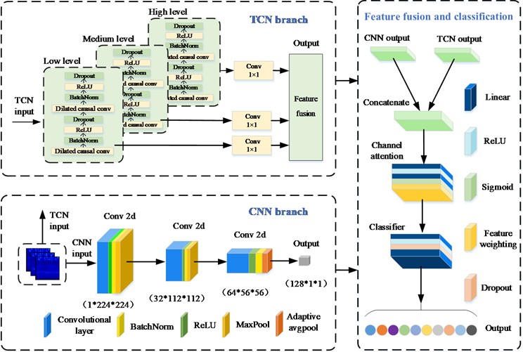
The frequency domain feature extraction branch adopts a three-layer CNN architecture with 32, 64 and 128 channels, respectively. As shown in Fig. 5, each convolutional block consists of a convolutional layer, a batch normalization layer and a ReLU activation function. The first two convolutional blocks are connected to a max pooling layer, and the spatial dimensions are halved to reduce the computational complexity. The final convolutional block is connected with an adaptive average pooling layer, which can capture the global frequency domain information while ensuring the consistency of the output dimension. The whole branch realizes the coding from local frequency domain to global semantic features through a hierarchical structure and finally outputs frequency domain features for feature fusion.

The time domain feature extraction branch adopts a three level TCN architecture, and each temporal block is composed of two dilated convolutional layers with batch normalization, ReLU activations, and dropout layers. In addition, the exponential expansion strategy is adopted to construct multi-scale temporal receptive fields and achieve long-term dependence modeling under limited network depth. In particular, the residual connection realizes the adaptive matching of the channel dimension through convolution, which ensures the effective propagation of the deep network gradient. The three-level dilated TCN is defined as:

6

\tilde{T} = {T C N}_{3} ({T C N}_{2} ({T C N}_{1} (t_{i}, d = 1), d = 2), d = 4),

where $t_{i} \in R^{T}$ denotes a single-node sequence. $\tilde{T} \in R^{N \times T}$ represents the joint output of $N$ nodes and $d$ denotes the dilation factor of the temporal convolution.

In order to integrate the temporal features $f_{t}$ from TCN and spectral features $f_{c}$ from CNN, a channel-wise attention mechanism is employed in this paper. The features are concatenated to form a unified representation $u = [f_{t}; f_{c}] .$ In an effort to dynamically prioritize informative channels, we compute an attention weight vector $α$ via a two-layer multi-layer perceptron:

7

α = σ (W_{2} δ (W_{1} u)),

where $δ$ is the ReLU activation, $σ$ is the Sigmoid function, and $W_{1}$ , $W_{2}$ are learning weight matrices. The final fused representation is obtained by re-calibrating the unified features $(v = α ⊙ u)$ , allowing the model to adaptively emphasize the most discriminative features from both time and frequency domains.

4. Experimental verification

Experiments are conducted on the Case Western Reserve University (CWRU) bearing dataset and the Harbin Institute of Technology (HIT) aero-engine bearing fault dataset to evaluate MCDCGAN-DPTAN with respect to diagnostic accuracy and robustness to class imbalance and noise. The CWRU dataset is employed to confirm diagnostic accuracy and robustness under imbalanced and noisy conditions, while the HIT dataset is introduced to assess cross-dataset generalization and robustness to class imbalance. All experiments are finished on a server equipped with an Intel Xeon Gold 6430 CPU and an NVIDIA RTX 4090 GPU, where the models are implemented in Python 3.12 and PyTorch 2.8.0 with CUDA 12.8.

4.1. Case 1: CWRU bearing dataset

4.1.1. CWRU dataset description

The rolling bearing datasets from CWRU are employed for building the benchmark datasets and validating the effectiveness of the proposed method [37]. The CWRU experimental platform is composed of a motor, a torque sensor, a dynamometer, a fan-end bearing and a drive-end bearing. The dataset consists of healthy and faulty signals acquired from the drive-end bearing under a 0 HP load (1797 RPM) condition. The experimental data is acquired at a sampling frequency of 12 kHz, covering inner race faults, ball faults, outer race faults and normal conditions, and the defect sizes of each fault are 7 mil, 14 mil and 21 mil, respectively. Table 2 provides a detailed description of the data.

Fig. 6The sliding window overlap sampling

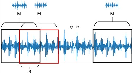
Table 2The data description of CWRU bearing datasets

Fault type	Normal	Inner race fault			Ball fault			Outer race fault
Fault diameter	–	0.007	0.014	0.021	0.007	0.014	0.021	0.007	0.014	0.021
Label	NL	IN_7	IN_14	IN_21	BALL_7	BALL_14	BALL_21	OUT_7	OUT_14	OUT_21

Fig. 7The time-frequency image of each fault sample

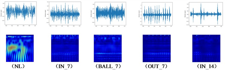
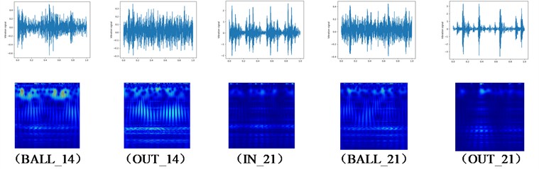
For the sake of obtaining sufficient sample data for model training, a sliding window overlapping sampling strategy is employed to extract samples from vibration signals under various operating conditions. As illustrated in Fig. 6, the sliding window length is set to 800, and the step size is 300, and each data type contains 400 samples. In this experiment, a balanced dataset and three unbalanced datasets are constructed to train the model. Specifically, different degrees of imbalanced datasets are created by selecting 50 %, 30 % and 20 % samples of each fault type respectively, and the number of normal samples remains unchanged. As shown in Table 3, Dataset A is a balanced dataset, and Datasets B, C, and D are unbalanced datasets. Subsequently, the intercepted one-dimensional vibration signal is transformed into a two-dimensional time-frequency representation by using CWT method, and the time-frequency images are shown in Fig. 7.

Table 3The datasets description of CWRU bearing datasets

Fault types	Dataset A	Dataset B	Dataset C	Dataset D
NL	100 %	100 %	100 %	100 %
IN_7	100 %	50 %	30 %	20 %
IN_14	100 %	50 %	30 %	20 %
IN_21	100 %	50 %	30 %	20 %
BALL_7	100 %	50 %	30 %	20 %
BALL_14	100 %	50 %	30 %	20 %
BALL_21	100 %	50 %	30 %	20 %
OUT_7	100 %	50 %	30 %	20 %
OUT_14	100 %	50 %	30 %	20 %
OUT_21	100 %	50 %	30 %	20 %

4.1.2. Generated images quality evaluation

In an effort to quantitatively evaluate the generated fault sample images, the FID, SSIM, and PSNR are adopted to analyze the experimental results. The FID index measures the consistency of the generated and real images at the distribution level, with lower values meaning greater similarity and diversity. The SSIM index quantifies the similarity of images by evaluating brightness, contrast, and structural information, with higher values indicating greater similarity. The PSNR index quantifies the image quality by the logarithmic ratio of the peak signal power to the mean square error, with higher values demonstrating reduced distortion and improved reconstruction fidelity. As shown in Fig. 8 and Table 4, the proposed MCDCGAN is far superior to the three classical models of CDCGAN, ACGAN and WGAN-GP in image generation quality, which further confirms the effectiveness of the proposed method.

Fig. 8The comparison of generated samples

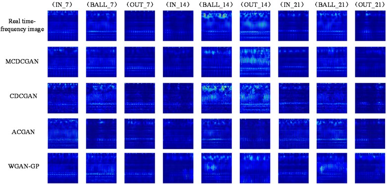
Additionally, this paper verifies the effectiveness of each module by removing each improved component in turn for ablation experiments. After independently training each variant, the corresponding generated images are evaluated, and the comprehensive evaluation results are shown in Table 5. With the successive addition of Wasserstein distance, spectral normalization, CBAM and self-attention modules, the image quality is significantly improved, which is manifested in the improvement of SSIM and PSNR indicators and the reduction of FID indicators. Especially, ablation experiments verify the effectiveness of each component of the proposed model in improving the quality of generated images.

Table 4The evaluation results of image quality

Fault types	MCDCGAN			CDCGAN			ACGAN			WGAN-GP
Fault types	SSIM	PSNR	FID	SSIM	PSNR	FID	SSIM	PSNR	FID	SSIM	PSNR	FID
IN_7	0.59	20.51	179.37	0.40	19.40	239.03	0.20	17.31	200.91	0.53	18.84	311.70
IN_14	0.49	18.08	189.01	0.35	17.05	195.15	0.26	15.37	249.03	0.53	16.51	314.29
IN_21	0.69	23.22	200.97	0.54	22.04	248.67	0.30	18.79	237.41	0.67	22.20	376.22
BALL_7	0.72	22.67	217.74	0.52	21.73	305.27	0.15	9.09	384.72	0.57	17.95	288.62
BALL_14	0.56	17.93	184.44	0.31	13.71	218.62	0.24	17.14	173.43	0.46	15.75	215.15
BALL_21	0.38	15.19	186.00	0.27	14.58	194.34	0.22	14.07	294.64	0.40	13.90	312.33
OUT_7	0.66	21.19	195.47	0.50	20.76	311.29	0.24	18.40	182.16	0.51	17.83	233.55
OUT_14	0.52	18.83	133.26	0.37	18.34	248.79	0.24	17.30	184.72	0.55	17.46	261.77
OUT_21	0.74	22.75	230.78	0.59	21.45	360.69	0.34	19.67	173.17	0.25	7.16	388.60
Mean	0.59	20.04	157.73	0.43	18.79	223.53	0.24	16.53	158.07	0.50	16.29	246.42

Table 5The result of ablation experiments

Model	SSIM	PSNR	FID
CDCGAN	0.4301	18.78	223.53
WCDDCGAN	0.5678	19.12	233.00
WCDCGAN (With SN)	0.5751	18.99	229.89
CBAM-WCDCGAN (SN)	0.5758	19.79	218.29
MCDCGAN	0.5946	20.04	157.72

4.1.3. Fault diagnosis analysis

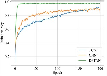
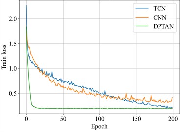
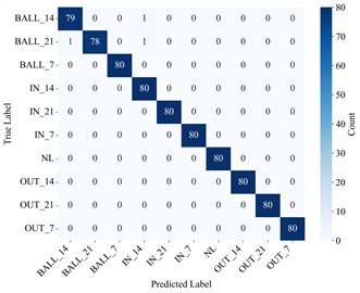
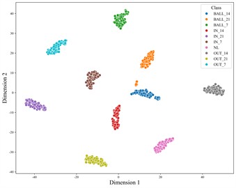
In order to evaluate the fault classification performance of the proposed DPTAN model, this paper conducts comparative experiments among TCN, CNN and DPTAN based on Dataset A, focusing on the analysis of training loss, accuracy trends and fault classification performance. As shown in Fig. 9, the DPTAN model exhibits a faster convergence rate and a more stable training process, and the training accuracy is steadily improved and finally reaches the highest level in the comparison model, which indicates that the DPTAN model is superior to the CNN and TCN models in terms of training efficiency and classification accuracy. As quantitatively summarized in Table 6, DPTAN achieves an accuracy of 99.63 % on the balanced CWRU Dataset A, outperforming the CNN baseline at 98.37 % and the TCN baseline at 97.13 % by a clear margin. In addition, DPTAN yields consistently high and well-aligned Precision, Recall, and F1-score, reaching 99.63 %, 99.63 %, and 99.62 %, respectively. The consistency between Precision, Recall, and F1-score reflects a well-balanced classification behavior. In Fig. 10, the confusion matrix and t-SNE plot jointly indicate clear class separability, with only minor confusion among similar categories. This observation aligns with the high Accuracy and F1-score reported in Table 6.

Fig. 9The comparison of model training loss and training accuracy

a) Accuracy curves

b) Loss curves

In order to further verify the effectiveness of the proposed method, this paper conducts a comparative test of the other two methods on the same datasets. The first method is trained directly on the original imbalanced datasets, and the second method is based on CDCGAN for data augmentation. Table 7 summarizes the classification accuracy of all methods on Dataset B, C and D. With the aggravation of class imbalance, MCDCGAN significantly improves the classification performance of DPTAN. The accuracy increases from 94.09 % to 98.88 % on Dataset B, from 88.51 % to 98.62 % on Dataset C, and from 81.25 % to 97.75 % on Dataset D, with the corresponding F1-score rising from 93.64 % to 98.87 %, from 87.95 % to 98.61 %, and from 81.25 % to 97.74 %, respectively. Moreover, MCDCGAN-based augmentation yields higher accuracy and F1-score than the CDCGAN-based strategy on Datasets B-D, indicating stronger robustness to class imbalance.

Fig. 10Confusion matrix and t-SNE visualization of DPTAN on the balanced CWRU Dataset A

a) Confusion matrix

b) t-SNE visualization

Table 6Fault diagnosis performance on the balanced CWRU Dataset A

Fault types	Accuracy (%)	Precision (%)	Recall (%)	F1-score (%)
CNN	98.37	98.40	98.38	98.37
TCN	97.13	97.44	97.13	97.10
DPTAN	99.63	99.63	99.63	99.62

Table 7Performance comparison of augmentation strategies on the imbalanced CWRU datasets

Method	Dataset B (Acc/F1) (%)	Dataset C (Acc/F1) (%)	Dataset D (Acc/F1) (%)
DPTAN (Imbalanced)	94.0/93.64	88.51/87.95	81.25/81.25
CDCGAN+DPTAN	97.38/97.33	97.12/97.10	96.88/96.86
MCDCGAN+DPTAN	98.88/98.87	98.62/98.61	97.75/97.74

4.1.4. Noise robustness analysis

In real-world industrial environments, acquired vibration signals are frequently contaminated by background noises. For the purpose of rigorously evaluating the robustness of the proposed diagnostic model against such interference, a series of noisy datasets are constructed by injecting Gaussian white noises with varying signal-to-noise ratios (SNRs) into the original CWRU data. Specifically, six SNR levels (–4 dB, –2 dB, 0 dB, 2 dB, 4 dB, and 6 dB) are selected for generating the corresponding noisy vibration data. Fig. 11 visualizes the waveform degradation under different noise levels. The CWT results in Fig. 12 reveal that low-SNR conditions blur time-frequency energy distributions, masking fault-related frequency bands.

In order to ensure statistical reliability, five independent trials are conducted at each SNR level. Table 8 lists the diagnostic performance metrics of the proposed method under different SNRs. As depicted in Fig. 13, as the SNR increases from –4 dB to 6 dB, the average diagnostic accuracy of the model progressively rises from 90.25 % to 98.50 %, demonstrating excellent noise robustness. Compared with other models, the proposed DPTAN method performs significantly better than traditional single-branch networks (e.g., CNN, TCN), especially under low SNR conditions. Notably, in severe noise environments, where SNR ≤ 0 dB, the proposed method retains high diagnostic precision, whereas the performance of comparative models declines significantly.

Fig. 11Signal waveforms with different SNRs

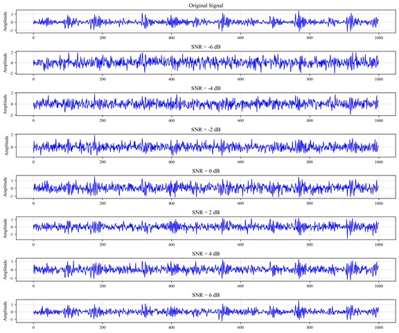
Fig. 12Time-frequency images of vibration signals under different SNRs

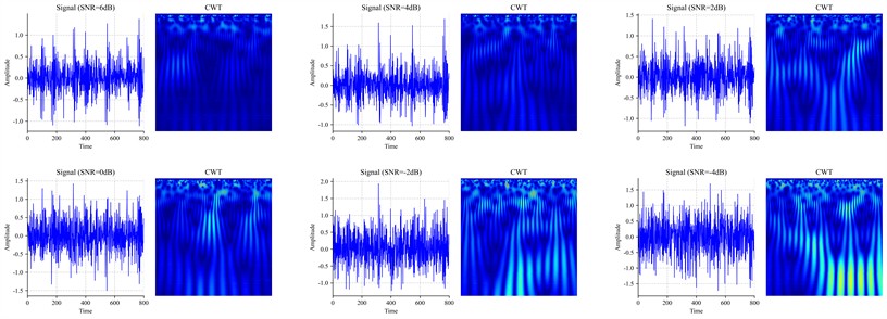
Fig. 13Average diagnostic accuracy of baseline methods under varying SNRs

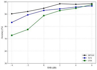
Table 8Fault diagnosis performance under different SNRs on the CWRU datasets

SNR (dB)	Accuracy (%)	Precision (%)	Recall (%)	F1-score (%)
6 dB	98.50	98.56	98.50	98.49
4 dB	98.00	98.06	98.00	97.98
2 dB	98.38	98.37	98.38	98.37
0 dB	94.75	94.95	94.75	94.73
–2 dB	92.13	92.14	92.13	92.09
–4 dB	90.25	90.39	90.25	90.25

4.2. Case 2: HIT bearing dataset

4.2.1. HIT dataset description

To further assess the generalization capability and class-imbalance robustness, experiments are conducted on the HIT aero-engine bearing dataset [38]. In this experiment, vibration signals under the operating condition of 4400 rpm (LP) and 5280 rpm (HP) are selected, covering three fault types including normal, inner-race fault, and outer-race fault. Following the same data processing pipeline as in the CWRU case study, one balanced dataset and three unbalanced datasets with varying imbalance ratios (50 %, 30 %, and 20 %) are constructed to evaluate the proposed model robustness. The detailed configuration of these datasets is summarized in Table 9. As shown in Fig. 14, the raw 1D vibration sequences are converted into 2D time-frequency spectrograms via CWT to serve as model inputs.

Table 9The datasets description of HIT bearing datasets

Fault types	Label	Dataset A	Dataset B	Dataset C	Dataset D
Normal	0	100 %	100 %	100 %	100 %
Inner ring	1	100 %	50 %	30 %	20 %
Outer ring	2	100 %	50 %	30 %	20 %

Fig. 14Vibration signals and their time–frequency images of different fault types

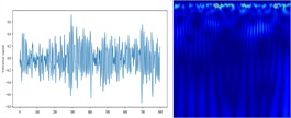
a) Normal

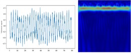
b) Inner ring

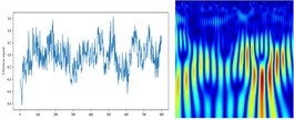
c) Outer ring

4.2.2. Cross-dataset fault diagnosis results on HIT

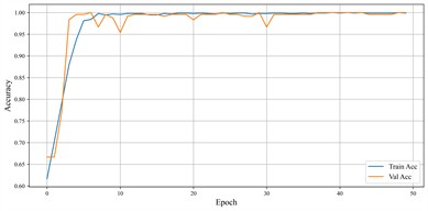
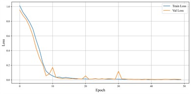
This subsection reports the diagnostic results on the HIT dataset to evaluate the cross-dataset generalization of the proposed method under distribution shift. This experiment adopts the same training setting as the CWRU experiment, ensuring that the observed performance faithfully reflects cross-dataset distribution shift. The training and validation accuracy and loss curves for the balanced Dataset A are shown in Fig. 15. The proposed DPTAN converges rapidly within the first 8-10 epochs and consistently maintains high accuracy with low loss throughout training. Table 10 further compares DPTAN with CNN and TCN baselines on HIT Dataset A. Overall, DPTAN achieves perfect performance on Dataset A, reaching 100 % accuracy and simultaneously obtaining 100 % Precision, 100 % Recall, and a 100 % F1-score, thereby outperforming the CNN and TCN baselines across all metrics.

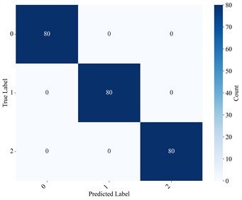
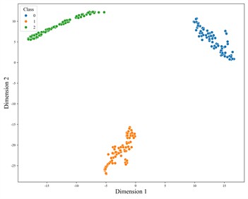
To provide a more intuitive assessment of the classification behavior, the confusion matrix and the corresponding t-SNE visualization of the learned feature representations are jointly presented in Fig. 16. As shown in Fig. 16(a), all test samples are correctly assigned to their ground-truth categories, and no noticeable confusion is observed among different fault conditions. Fig. 16(b) shows t-SNE-extracted features before the final classifier, where data from distinct fault types form compact, well-separated clusters with obvious decision boundaries. These results indicate that DPTAN learns highly discriminative representations and preserves robust class separability under cross-dataset distribution shift.

Fig. 15Learning curves of DPTAN on the balanced HIT Dataset A

a) Accuracy curves

b) Loss curves

Table 10Fault diagnosis performance on the balanced HIT Dataset A

Fault types	Accuracy (%)	Precision (%)	Recall (%)	F1-score (%)
CNN	97.88	97.63	97.62	97.97
TCN	98.39	98.48	98.35	98.36
DPTAN	100	100	100	100

Fig. 16Confusion matrix and t-SNE visualization of DPTAN on the balanced HIT Dataset A

a) Confusion matrix

b) t-SNE visualization

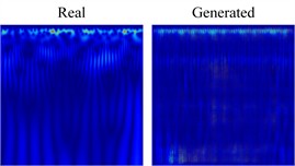
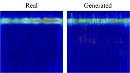
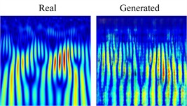
In order to mitigate the class-imbalance issue, Fig. 17 presents representative real samples and MCDCGAN-generated time–frequency images for several fault categories. Table 11 summarizes the results under class-imbalanced settings on Datasets B to D. One hand the noticeable gap between the imbalanced DPTAN baseline and the augmentation-assisted variants indicates that class imbalance can substantially degrade diagnostic performance. On the other hand, the MCDCGAN-augmented scheme consistently yields higher Accuracy and F1-score than the CDCGAN-based augmentation, suggesting a stronger mitigation effect against imbalance-induced performance deterioration under distribution shift.

Fig. 17Real and MCDCGAN-generated samples on HIT

a) Normal

b) Inner ring

c) Outer ring

Table 11Performance comparison of augmentation strategies on the imbalanced HIT datasets

Method	Dataset B (Acc/F1) (%)	Dataset C (Acc/F1) (%)	Dataset D (Acc/F1) (%)
DPTAN (Imbalanced)	96.75/96.25	91.56/89.06	86.61/85.53
CDCGAN+DPTAN	98.96/98.65	98.13/97.08	96.88/96.46
MCDCGAN+DPTAN	99.68/99.58	99.58/99.58	99.27/99.17

4.3. Algorithm complexity analysis

This paper assesses the efficiency of the proposed framework by counting the total number of training parameters for each module and calculating the number of floating-point operations (FLOPs) required to complete one forward propagation. The total parameter count is obtained by summing the weights and biases across all learnable layers. For a standard two-dimensional convolutional layer with a kernel size of $K \times K$ , $C_{i n}$ denotes input channels, and $C_{o u t}$ on behalf of output channels, the number of parameters is $K^{2} \cdot C_{i n} \cdot C_{o u t} + C_{o u t}$ . The computational cost, measured in FLOPs, is derived based on the output feature map dimensions. For the same 2D convolutional layer with output size $H \times W$ , the FLOPs are approximated as:

8

{F L O P s}_{c o n v 2 d} \approx 2 \cdot H \cdot W \cdot K^{2} {\cdot C}_{i n} \cdot C_{o u t} .

Similarly, for the one-dimensional temporal convolution in the TCN branch with sequence length $L$ and kernel size $K_{t}$ , the FLOPs scale can be written as:

9

{F L O P s}_{c o n v 1 d} \approx 2 \cdot L \cdot K_{t} \cdot C_{i n} \cdot C_{o u t} .

Based on above formulations, the detailed complexity metrics are presented in Table 12. Although the MCDCGAN generator incurs a substantial offline cost (13.53 GFLOPs) for high-fidelity generation, the proposed DPTAN remains highly efficient for real-time diagnosis with 0.77 M parameters and 1.12 GFLOPs.

Table 12Estimated complexity of the MCDCGAN-DPTAN framework

Model	Module	Parameters (M)	FLOPs (G)
MCDCGAN	Generator	12.57	13.53
MCDCGAN	Discriminator	4.55	0.18
DPTAN	TCN Branch	0.25	0.11
	CNN Branch	0.09	0.95
	Fusion Block	0.15	< 0.01
	Classifier	0.10	< 0.01
	Total	0.77	1.12

5. Conclusions

A bearing fault diagnosis method based on MCDCGAN and DPTAN has been proposed in this paper. Firstly, the bearing fault vibration signal has been preprocessed by adopting the CWT method. Moreover, a MCDCGAN model has been designed to effectively address the problem of data imbalance by combining CBAM, self-attention mechanism, Wasserstein distance and spectral normalization. Furthermore, by integrating CNN and TCN, a DPTAN model has been designed to achieve accurate bearing fault classification. Finally, experimental verification has been carried out by employing the CWRU and HIT datasets. The experimental results have shown that the proposed method is effective and practical for bearing fault diagnosis under class imbalance and noisy conditions.

References

G. Li, M. Wei, D. Wu, Y. Cheng, J. Wu, and J. Yan, “Zero-sample fault diagnosis of rolling bearings via fault spectrum knowledge and autonomous contrastive learning,” Expert Systems with Applications, Vol. 275, p. 127080, Feb. 2025, https://doi.org/10.1016/j.eswa.2025.127080

Publisher
P. Zhu et al., “Deep spiking transfer learning for rotating machinery fault diagnosis,” Mechanical Systems and Signal Processing, Vol. 241, p. 113499, Oct. 2025, https://doi.org/10.1016/j.ymssp.2025.113499

Publisher
L. Xiao, Y. Chen, M. Wang, H. Zhao, and Q. Zhou, “Multisource-multitarget partial domain adaptation for bearing fault diagnosis,” IEEE Internet of Things Journal, Vol. 12, No. 11, pp. 15897–15910, Jun. 2025, https://doi.org/10.1109/jiot.2025.3529953

Publisher
J. Zhuang, Y. Cao, M. Jia, X. Zhao, and Q. Peng, “Fault diagnosis of bearings using a two-stage transfer alignment approach with semantic consistency and entropy loss,” Expert Systems with Applications, Vol. 226, p. 120274, Apr. 2023, https://doi.org/10.1016/j.eswa.2023.120274

Publisher
T.-T. Vo, M.-K. Liu, and M.-Q. Tran, “Harnessing attention mechanisms in a comprehensive deep learning approach for induction motor fault diagnosis using raw electrical signals,” Engineering Applications of Artificial Intelligence, Vol. 129, p. 107643, Dec. 2023, https://doi.org/10.1016/j.engappai.2023.107643

Publisher
Z. Zhu et al., “A review of the application of deep learning in intelligent fault diagnosis of rotating machinery,” Measurement, Vol. 206, p. 112346, Dec. 2022, https://doi.org/10.1016/j.measurement.2022.112346

Publisher
V. Sinitsin, O. Ibryaeva, V. Sakovskaya, and V. Eremeeva, “Intelligent bearing fault diagnosis method combining mixed input and hybrid CNN-MLP model,” Mechanical Systems and Signal Processing, Vol. 180, p. 109454, Jun. 2022, https://doi.org/10.1016/j.ymssp.2022.109454

Publisher
M. Wang, W. Wang, X. Zhang, and H. H.-C. Iu, “A new fault diagnosis of rolling bearing based on Markov transition field and CNN,” Entropy, Vol. 24, No. 6, p. 751, May 2022, https://doi.org/10.3390/e24060751

Publisher
Z. Jiang, Y. Li, J. Gao, and C. Wu, “A fault detection of aero-engine rolling bearings based on CNN-BiLSTM network integrated cross-attention,” Measurement Science and Technology, Vol. 35, No. 12, p. 126116, Dec. 2024, https://doi.org/10.1088/1361-6501/ad7622

Publisher
R. Wang, E. Dong, Z. Cheng, Z. Liu, and X. Jia, “Transformer-based intelligent fault diagnosis methods of mechanical equipment: A survey,” Open Physics, Vol. 22, No. 1, May 2024, https://doi.org/10.1515/phys-2024-0015

Publisher
H. Wang, W. Zhang, C. Han, Z. Fu, and L. Song, “A bearing fault diagnosis method with an improved residual Unet diffusion model under extreme data imbalance,” Measurement Science and Technology, Vol. 35, No. 4, p. 046113, Apr. 2024, https://doi.org/10.1088/1361-6501/ad1708

Publisher
M. Ye, X. Yan, X. Hua, D. Jiang, L. Xiang, and N. Chen, “MRCFN: A multi-sensor residual convolutional fusion network for intelligent fault diagnosis of bearings in noisy and small sample scenarios,” Expert Systems with Applications, Vol. 259, p. 125214, Aug. 2024, https://doi.org/10.1016/j.eswa.2024.125214

Publisher
X. Yan, D. Jiang, L. Xiang, Y. Xu, and Y. Wang, “CDTFAFN: A novel coarse-to-fine dual-scale time-frequency attention fusion network for machinery vibro-acoustic fault diagnosis,” Information Fusion, Vol. 112, p. 102554, Dec. 2024, https://doi.org/10.1016/j.inffus.2024.102554

Publisher
M. Ye, X. Yan, D. Jiang, and N. Chen, “A multi-branch attention coupled convolutional domain adaptation network for bearing intelligent fault recognition under unlabeled sample scenarios,” Applied Soft Computing, Vol. 174, p. 113053, Mar. 2025, https://doi.org/10.1016/j.asoc.2025.113053

Publisher
M. Ye, X. Yan, D. Jiang, L. Xiang, and N. Chen, “MIFDELN: A multi-sensor information fusion deep ensemble learning network for diagnosing bearing faults in noisy scenarios,” Knowledge-Based Systems, Vol. 284, p. 111294, Dec. 2023, https://doi.org/10.1016/j.knosys.2023.111294

Publisher
X. Yan, X. Jin, D. Jiang, and L. Xiang, “Remaining useful life prediction of rolling bearings based on CNN-GRU-MSA with multi-channel feature fusion,” Nondestructive Testing and Evaluation, pp. 1–26, Sep. 2024, https://doi.org/10.1080/10589759.2024.2408670

Publisher
L. Zeng, J. Jian, X. Chang, and S. Wang, “A meta-learning method for few-shot bearing fault diagnosis under variable working conditions,” Measurement Science and Technology, Vol. 35, No. 5, p. 056205, May 2024, https://doi.org/10.1088/1361-6501/ad28e7

Publisher
W. Cui et al., “Fault diagnosis of rolling bearings in primary mine fans under sample imbalance conditions,” Entropy, Vol. 25, No. 8, p. 1233, Aug. 2023, https://doi.org/10.3390/e25081233

Publisher
H. Shi, Y. Zhang, Y. Chen, S. Ji, and Y. Dong, “Resampling algorithms based on sample concatenation for imbalance learning,” Knowledge-Based Systems, Vol. 245, p. 108592, Mar. 2022, https://doi.org/10.1016/j.knosys.2022.108592

Publisher
I. J. Goodfellow et al., “Generative adversarial networks,” arXiv, Jun. 2014, https://doi.org/10.48550/arxiv.1406.2661

Publisher
Y. Zhang et al., “Fault diagnosis based on C-DCGAN for rolling bearing,” in Global Reliability and Prognostics and Health Management (PHM-Yantai), Oct. 2022, https://doi.org/10.1109/phm-yantai55411.2022.9941993

Publisher
X. Xu, X. Chen, and Y. Zhao, “Data imbalance bearing fault diagnosis based on fusion attention mechanism and global feature cross GAN network,” Measurement Science and Technology, Vol. 35, No. 10, p. 106136, Oct. 2024, https://doi.org/10.1088/1361-6501/ad64f5

Publisher
Z. Men, Y. Li, L. Gao, and Z. Zhang, “Fault diagnosis method for railway wagon bearings under imbalanced dataset based on improved ACWGAN,” Nonlinear Dynamics, Vol. 113, No. 12, pp. 14935–14962, Feb. 2025, https://doi.org/10.1007/s11071-025-10878-x

Publisher
Y. Li, X. Jiang, and J. Wu, “Rating entropy and its multivariate version,” Mechanical Systems and Signal Processing, Vol. 226, p. 112368, Jan. 2025, https://doi.org/10.1016/j.ymssp.2025.112368

Publisher
L. Jiang, C. Shi, H. Sheng, X. Li, and T. Yang, “Lightweight CNN architecture design for rolling bearing fault diagnosis,” Measurement Science and Technology, Vol. 35, No. 12, p. 126142, Dec. 2024, https://doi.org/10.1088/1361-6501/ad7a1a

Publisher
L. Ding and Q. Li, “Fault diagnosis of rotating machinery using novel self-attention mechanism TCN with soft thresholding method,” Measurement Science and Technology, Vol. 35, No. 4, p. 047001, Apr. 2024, https://doi.org/10.1088/1361-6501/ad1eb3

Publisher
R. N. Toma et al., “A bearing fault classification framework based on image encoding techniques and a convolutional neural network under different operating conditions,” Sensors, Vol. 22, No. 13, p. 4881, Jun. 2022, https://doi.org/10.3390/s22134881

Publisher
Y. Wu et al., “The fault diagnosis of rolling bearings based on FFT-SE-TCN-SVM,” Actuators, Vol. 14, No. 3, p. 152, Mar. 2025, https://doi.org/10.3390/act14030152

Publisher
L. Meng, Y. Su, X. Kong, T. Xu, X. Lan, and Y. Li, “Intelligent fault diagnosis of gearbox based on differential continuous wavelet transform-parallel multi-block fusion residual network,” Measurement, Vol. 206, p. 112318, Dec. 2022, https://doi.org/10.1016/j.measurement.2022.112318

Publisher
H. S. Kumar and G. Upadhyaya, “Fault diagnosis of rolling element bearing using continuous wavelet transform and K-nearest neighbour,” Materials Today: Proceedings, Vol. 92, pp. 56–60, 2023, https://doi.org/10.1016/j.matpr.2023.03.618

Publisher
M. Mehralian and B. Karasfi, “RDCGAN: unsupervised representation learning with regularized deep convolutional generative adversarial networks,” in 9th Conference on Artificial Intelligence and Robotics and 2nd Asia-Pacific International Symposium, pp. 31–38, 2019, https://doi.org/10.1109/aiar.2018.8769811

Publisher
C. Deng, Z. Deng, S. Lu, M. He, J. Miao, and Y. Peng, “Fault diagnosis method for imbalanced data based on multi-signal fusion and improved deep convolution generative adversarial network,” Sensors, Vol. 23, No. 5, p. 2542, Feb. 2023, https://doi.org/10.3390/s23052542

Publisher
L. Andéol, Y. Kawakami, Y. Wada, T. Kanamori, K.-R. Müller, and G. Montavon, “Learning domain invariant representations by joint Wasserstein distance minimization,” Neural Networks, Vol. 167, pp. 233–243, Jul. 2023, https://doi.org/10.1016/j.neunet.2023.07.028

Publisher
J. Mi, C. Ma, L. Zheng, M. Zhang, M. Li, and M. Wang, “WGAN-CL: a Wasserstein GAN with confidence loss for small-sample augmentation,” Expert Systems with Applications, Vol. 233, p. 120943, Jul. 2023, https://doi.org/10.1016/j.eswa.2023.120943

Publisher
M. Zhao, X. Pan, S. Xiao, Y. Zhang, C. Tang, and X. Wen, “Seismic data interpolation based on spectrally normalized generative adversarial network,” IEEE Transactions on Geoscience and Remote Sensing, Vol. 61, pp. 1–11, Aug. 2023, https://doi.org/10.1109/tgrs.2023.3301270

Publisher
S. Woo, J. Park, J.-Y. Lee, and I. S. Kweon, “CBAM: convolutional block attention module,” in Computer Vision, 2018, https://doi.org/10.1007/978-3-030-01234-2_1

Publisher
W. A. Smith and R. B. Randall, “Rolling element bearing diagnostics using the Case Western Reserve University data: a benchmark study,” Mechanical Systems and Signal Processing, Vol. 64-65, pp. 100–131, May 2015, https://doi.org/10.1016/j.ymssp.2015.04.021

Publisher
L. Hou et al., “Inter-shaft bearing fault diagnosis based on aero-engine system: a benchmarking dataset study,” Journal of Dynamics, Monitoring and Diagnostics, Vol. 2, No. 4, pp. 228–242, Aug. 2023, https://doi.org/10.37965/jdmd.2023.314

Publisher

About this article

Received

September 10, 2025

Accepted

May 31, 2026

Published

August 3, 2026

DOI

https://doi.org/10.21595/jme.2026.25374

Keywords

attention mechanism

bearing fault diagnosis

DPTAN

feature extraction

MCDCGAN

Acknowledgements

This work was supported in part by the National Natural Science Foundation of China under Grant 61803193, in part by the Natural Science Foundation of Shandong Province of China under Grant ZR2023QF027, in part by the Research Initiation Fund Project of Linyi University under Grant Z6122027 and in part by the Innovation Project of Linyi University under Grant 518240509.

Data Availability

The datasets generated during and/or analyzed during the current study are available from the corresponding author on reasonable request.

Author Contributions

Sen Zhang conceived the core idea, led the formal analysis, and drafted the manuscript. Le Yan developed the methodology and supported result interpretation. Zhaodong Liu conducted the experiments and implemented the software. Hao Ren provided methodological guidance, supervised the study, and reviewed the manuscript. Heng Lu assisted with experiments and software implementation.

Conflict of interest

The authors declare that they have no conflict of interest.

This is an open access article distributed under the Creative Commons Attribution License, which permits unrestricted use, distribution, and reproduction in any medium, provided the original work is properly cited.

S. Zhang, L. Yan, Z. Liu, H. Ren, and H. Lu, “A bearing fault diagnosis method based on MCDCGAN and DPTAN under data imbalance,” Journal of Measurements in Engineering, Vol. 14, No. 4, –20, Aug. 2026, https://doi.org/10.21595/jme.2026.25374

Copy Extrica

Copied to clipboard!

TY  - JOUR
DO  - 10.21595/jme.2026.25374
UR  - https://doi.org/10.21595/jme.2026.25374
TI  - A bearing fault diagnosis method based on MCDCGAN and DPTAN under data imbalance
T2  - Journal of Measurements in Engineering
AU  - Zhang, Sen
AU  - Yan, Le
AU  - Liu, Zhaodong
AU  - Ren, Hao
AU  - Lu, Heng
PY  - 2026
DA  - 2026/08/03
PB  - Extrica
VL  - 14
IS  - 4
SN  - 2335-2124
SN  - 2424-4635
ER  - 

Copy Ris

Copied to clipboard!

@article{doi_10.21595/jme.2026.25374,
  title = {A bearing fault diagnosis method based on MCDCGAN and DPTAN under data imbalance},
  author = {Zhang, Sen and Yan, Le and Liu, Zhaodong and Ren, Hao and Lu, Heng},
  journal = {Journal of Measurements in Engineering},
  year = {2026},
  month = {8},
  volume = {14},
  number = {4},
  doi = {10.21595/jme.2026.25374},
  url = {https://doi.org/10.21595/jme.2026.25374},
  publisher = {Extrica},
  issn = {2335-2124},
  eissn = {2424-4635},
}

Copy Bibtex

Copied to clipboard!

[1]S. Zhang, L. Yan, Z. Liu, H. Ren, and H. Lu, “A bearing fault diagnosis method based on MCDCGAN and DPTAN under data imbalance,” Journal of Measurements in Engineering, Aug. 2026, doi: 10.21595/jme.2026.25374.

Copy IEEE

Copied to clipboard!

Zhang, Sen, Le Yan, Zhaodong Liu, Hao Ren, and Heng Lu. “A bearing fault diagnosis method based on MCDCGAN and DPTAN under data imbalance.” Journal of Measurements in Engineering 14, no. 4 (2026). https://doi.org/10.21595/jme.2026.25374.

Copy Chicago

Copied to clipboard!