Reliability evaluation of SiC MOSFET with performance degradation under multiple conditions based on nonlinear wiener process

Li, Yaoheng; Zhang, Jinbao; Wang, Hui; Zhang, Jinle; Zhang, Haiquan; Zhao, Fuqiang

doi:10.21595/jme.2026.25806

Journal of Measurements in Engineering

Browse Journal

Submit article

Published: June 4, 2026

Check for updates

Reliability evaluation of SiC MOSFET with performance degradation under multiple conditions based on nonlinear wiener process

Yaoheng Li¹

Jinbao Zhang²

Hui Wang³

Jinle Zhang⁴

Haiquan Zhang⁵

Fuqiang Zhao⁶

^{1, 2, 4, 5, 6}China North Vehicle Research Institute, Beijing, China

³Urban Safety Engineering, Beijing Polytechnic College, Beijing, China

Corresponding Author:

Hui Wang

Cite the article Download PDF

Article in Press

Downloads 0

Abstract

A reliability evaluation method for SiC MOSFET components based on the nonlinear Wiener process is proposed using small-sample threshold voltage degradation data under multiple operating conditions. In this method, the exponential function and power function are respectively used to characterize the influences of influencing factor parameters and time effects on the drift coefficient, thereby establishing a mathematical model capable of describing the degradation behavior of SiC MOSFET components. Based on the threshold voltage degradation data of 35 SiC MOSFET component samples, Limited-memory Broyden-Fletcher-Goldfarb-Shanno with Bound constraints (L-BFGS-B) is employed for parameter estimation. Meanwhile, the Bootstrap method is adopted to quantify the uncertainties of the initial degradation amount and influencing factor parameters under small-sample conditions. Through the Monte Carlo simulation method, the reliability evaluation of SiC MOSFET components is conducted under the designed operating conditions, and accurate reliability evaluation results, as well as their confidence intervals are obtained. The results demonstrate that the proposed nonlinear Wiener process model can effectively capture the degradation characteristics of SiC MOSFET components under different operating conditions, providing a scientific basis for further reliability evaluation and life prediction of power electronic equipment.

1. Introduction

As core components of modern power electronic systems, SiC MOSFET components are widely used in key fields such as renewable energy generation, smart grids, electric vehicles, and industrial frequency converters [1-2]. Their reliability directly affects the operational safety, life cycle, and economic benefits of the entire equipment system [3-4]. However, SiC MOSFET components often operate under complex electro-thermal stress conditions in multi-field coupling environments, leading to gradual performance degradation over time and eventual functional failure [5-6]. Therefore, accurate reliability evaluation of SiC MOSFET components is of great theoretical and engineering significance, enabling predictive maintenance, system design optimization, and safe operation [7-9].

Traditional reliability evaluation methods, such as accelerated life testing, typically require large quantities of failure samples, involve long test cycles and high costs, and struggle to accurately represent the degradation process under actual multi-condition operation. In contrast, the methods based on performance degradation data can utilize the performance parameter change trajectory of components during the degradation process to evaluate and predict their reliability before complete product failure, especially suitable for high-reliability and long-life semiconductor devices [10-12]. The reliability evaluation methods based on performance degradation data include degradation path uncertainty modeling [13], pseudo failure life method [14], general degradation modeling method [15], and stochastic process, etc.

In recent years, degradation modeling based on stochastic processes has become one of the mainstream methods in reliability research, including Wiener processes [16-17], gamma processes [18-20], and inverse Gaussian processes [21]. While gamma and inverse Gaussian processes assume strictly positive degradation increments – suitable for irreversible processes such as crack growth or wear – they cannot capture non-monotonic degradation behaviors. The Wiener process incorporates a random diffusion term $σ B (t)$ based on Brownian motion, and allows for temporary “recovery” phenomena in the degradation path, making it suitable for modeling non-monotonic degradation trajectories. Owing to its mathematical tractability, the Wiener process is widely used to describe performance degradation in semiconductor devices, lasers, and other products.

The core advantage of the Wiener process lies in its ability to describe non-monotonic degradation, excellent mathematical properties, easy implementation, and strong model interpretability [10-12]. The core parameters of the model – drift coefficient $μ$ and diffusion coefficient $σ$ – can be efficiently estimated via maximum likelihood estimation with analytical solutions. The product's lifetime follows an inverse Gaussian distribution, which has well-defined probability density and cumulative distribution functions. Furthermore, the Wiener process readily accommodates covariate influences, e.g., temperature, voltage, vibration, by modeling $μ$ as a function of these stresses, facilitating accelerated degradation testing. It also supports the inclusion of random effects to account for unit-to-unit variability, enhancing overall reliability characterization. The parameters $μ$ and $σ$ have intuitive physical interpretations: $μ$ represents the average degradation rate, while $σ$ reflects uncertainty or fluctuation intensity in the degradation process.

Many researchers have explored these properties of the Wiener process. Some studies have introduced time-varying drift or diffusion coefficients to construct nonlinear Wiener processes, better capturing nonlinear degradation effects [22-23]. Other efforts focus on reliability modeling under multiple stresses, often employing acceleration models such as the Arrhenius model to relate stress levels to model parameters [24-27]. However, existing studies still need further exploration for reliability evaluation of SiC MOSFET components performance degradation: (1) insufficient consideration of variability in initial degradation values and failure threshold values among individual units, affecting model accuracy [28-29]; (2) neglect of parameter estimation uncertainty under small-sample conditions, leading to over-optimistic evaluation results without confidence intervals; and (3) coupling of environmental stress and time effects within the same function, which obscures their independent physical mechanisms. In fact, the time effect mainly reflects the inherent degradation processes such as material aging and defect accumulation inside the device, while environmental stress (such as temperature and voltage) affects the degradation rate by accelerating or slowing down these processes. Separating the two models could clearly distinguish the contribution of inherent device lifespan and environmental acceleration factor, support extrapolation of degradation laws between different operating conditions, and guide the stress level design for accelerated degradation testing.

To address these issues, this paper focuses on SiC MOSFET reliability evaluation with small samples under multiple operating conditions. The main contributions are as follows: Based on threshold voltage degradation data of SiC MOSFETs, a Wiener process degradation model that accounts for both multiple operating conditions and temporal nonlinearity is established, along with an uncertainty quantification method for small-sample data. Using the estimated model parameters, the first passage time distribution under designed conditions is predicted via Monte Carlo simulation, and key reliability metrics such as the reliability function and confidence intervals are provided, offering a quantitative basis for engineering decision-making.

2. The nonlinear Wiener process with parameter estimation

2.1. The nonlinear Wiener process model

For the performance degradation process of SiC MOSFET, the following nonlinear Wiener process model is established:

1

X (t) = X_{0} + μ (z) \int_{0}^{t} τ^{γ} d τ + σ B (t),

where $X (t)$ is the degradation quantity at time $t$ ; the initial degradation quantity $X_{0}$ as a random variable is independent and identically distributed; $γ > 0$ is the power exponent of time; $σ > 0$ is the diffusion coefficient, which is assumed not to change with time and operating conditions; $B (t)$ is standard Brownian motion; $μ (z)$ is a drift coefficient function that depends on influencing factors $z$ , expressed in the exponential form:

2

μ (z) = e x p (β_{0} + \sum_{j = 1}^{C} β_{j} z_{j}),

where $C$ is the number of influencing factor parameters, and $β = [β_{0}, β_{1}, \dots β_{C}]$ is the coefficient of influencing factors.

2.2. Parameter estimation

Due to manufacturing variations, initial performance values may differ even among components from the same batch. Measurement errors and environmental fluctuations also contribute to variability in initial readings. Therefore, the initial degradation is modeled as a random variable following a normal distribution:

3

X_{0} ~ N (μ_{0}; σ_{0}^{2}),

where $μ_{0}$ and $σ_{0} > 0$ respectively are the mean and the standard deviation of $X_{0}$ .

For the $k$ th sample, the initial degradation contribution is:

4

f_{0 k} = \frac{1}{σ_{0} \sqrt{2 π}} e x p [- \frac{{(x_{0 k} - μ_{0})}^{2}}{2 σ_{0}^{2}}] .

Assuming that the threshold voltage under different operating conditions follows the same distribution. For the degradation increment $∆ X = X (t_{i}) - X (t_{i - 1})$ within the time interval $[t_{i - 1}, t_{i}]$ , it follows a normal distribution:

5

∆ X ~ N (μ_{∆ X} (z, t_{i}), σ^{2} (t_{i} - t_{i - 1})),

where $μ_{∆ X} (z, t_{i})$ is the mean of $∆ X$ from time $t_{i - 1}$ to time $t_{i}$ and it is defined as:

6

μ_{∆ X} (z, t_{i}) = μ (z) \int_{t_{i - 1}}^{t_{i}} τ^{γ} d τ = e x p (β_{0} + \sum_{j = 1}^{C} β_{j} z_{j}) \times \frac{t_{i}^{γ + 1} - t_{i - 1}^{γ + 1}}{γ + 1} .

The corresponding probability density function is:

7

f (∆ X) = \frac{1}{σ \sqrt{2 π (t_{i} - t_{i - 1})}} e x p [- \frac{{(∆ X - μ_{∆ X} (z, t_{i}))}^{2}}{2 σ^{2} (t_{i} - t_{i - 1})}] .

For the $k$ th sample, its complete likelihood function is the product of the initial value probability and the incremental degradation probability over all time intervals:

8

L_{k} = f_{0 k} \times \prod_{i = 2}^{n_{k}} f ({∆ X}_{k i}),

where $n_{k}$ is the number of observations of the $k$ th sample.

The joint likelihood function for all $K$ samples is:

9

L = \prod_{k = 1}^{K} L_{k} .

The logarithmic likelihood function is:

10

l = \sum_{k = 1}^{K} [l n f_{0 k} + \sum_{i = 2}^{n_{k}} l n f ({∆ X}_{k i})] .

The parameters that need to be estimated include: the distribution parameters $μ_{0}$ , $σ_{0}$ of initial values $X_{0}$ ; coefficients of the influencing factors $β = [β_{0}, β_{1}, \dots β_{C}]$ ; the time power exponent $γ$ ; the diffusion coefficient $σ$ . The total parameters to be estimated are integrated as $Θ = [{μ_{0}, σ_{0}, β}_{0}, β_{1}, \dots β_{C}, γ, σ]$ .

Parameters are estimated by maximizing the logarithmic likelihood function:

11

\hat{Θ} = \arg \max_{Θ} l (Θ) .

Due to the complexity of the model, L-BFGS-B is used for parameter solving.

For small sample data, the Bootstrap method is used to quantify the uncertainty of parameter estimation. Extract $B$ Bootstrap sample sets with replacement from the original sample $S$ :

12

S^{(k)} = B o o t s t r a p (S), k = 1, 2, \dots, B,

In this paper, $B$ is set as 50 based on a trade-off between convergence analysis and computational efficiency, ensuring the stability of the parameter estimates.

Estimate the parameters of each Bootstrap sample set to obtain:

13

{\hat{Θ}}^{(k)} = \arg \max_{Θ} l (Θ |S^{(k)})

And then calculate the confidence interval of parameters based on Bootstrap estimation values.

The standard error estimate for the $j$ -th parameter is:

14

S E ({\hat{θ}}_{j}) = \sqrt{\frac{1}{B - 1} \sum_{b = 1}^{B} {({\hat{θ}}_{j, b} - {\bar{θ}}_{j})}^{2}},

where ${\bar{θ}}_{j} = \frac{1}{B} \sum_{b = 1}^{B} {\hat{θ}}_{j, b}$ . The final 100( $1 - α$ ) % confidence interval for the $j$ -th parameter is $[{\hat{θ}}_{j}^{(α / 2)}, {\hat{θ}}_{j}^{(1 - α / 2)}]$ , in which ${\hat{θ}}_{j}^{(α / 2)}$ and ${\hat{θ}}_{j}^{(1 - α / 2)}$ respectively represent the $α / 2$ and $1 - α / 2$ quantiles of the Bootstrap estimate values ${\hat{θ}}_{j, 1}, {\hat{θ}}_{j, 2}, \dots, {\hat{θ}}_{j, B}$ .

3. Reliability evaluation model

The lifetime of a component is defined as the time when the degradation first exceeds the failure threshold:

15

T_{f} = i n f \{t > 0 : X (t) \geq D_{f}\},

where $D_{f}$ is the failure threshold. Considering the randomness of the initial value and the effects of influencing factors, the Monte Carlo simulation method is adopted as follows:

(1) Randomly generate initial values $x_{0}$ from the initial value distribution $N (μ_{0}; σ_{0}^{2})$ .

(2) With each group of estimated parameters, simulate the nonlinear Wiener process path until $X (t) \geq D_{f}$ .

(3) Record the first passage time $T_{f}$ .

(4) Repeat multiple times to obtain the empirical distribution of the first passage time.

Based on the Monte Carlo simulation results, the estimated reliability function is:

16

R (t) = \frac{1}{T N u m} \sum_{j = 1}^{T N u m} 1_{\{T_{f}^{(j)} > t\}},

where $T_{f}^{(j)}$ is the first passage time of the $j$ -th simulation; $T N u m$ is the total number of simulations, which is set as 10000 in this paper.

4. SiC MOSFET performance degradation test and data analysis

4.1. Experiment test

The experimental testing platform is shown in Fig. 1. A total of 35 samples are tested under 15 operating conditions, as listed in Table 1. Each operating condition involves 7 influencing factors, including gate turn-on voltage (V), gate turn-off voltage (V), duty cycle (%), switching frequency (kHz), on resistance (R), off resistance (R), temperature (℃), with the corresponding coefficients from $β_{1}$ to $β_{7}$ sequentially.

Fig. 1Test bench of the SiC MOSFET. Photo by Yaoheng Li, at China North Vehicle Research Institute in China on June 2025

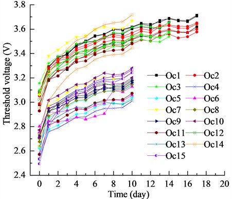
To eliminate the influence of dimensions and units of the influencing factors, a normalization process is applied. The threshold voltage degradation data are collected on a daily basis, and the resulting degradation paths are shown in Fig. 2, in which the horizontal axis represents time in days, the vertical axis shows the threshold voltage degradation in volts, and different colors represent different operating conditions. A clear upward trend in threshold voltage over time is observed. From the degradation paths in Fig. 2, it can be seen that the threshold voltage of some samples was close to the 4 V at the end of the test, while the degradation trend of all samples indicates that they will cross this threshold in the foreseeable future, ensuring the observability of the failure time.

Table 1SiC MOSFET test conditions

Operating conditions	Gate turn-on voltage (V)	Gate turn-off voltage (V)	Duty cycle (%)	Switching frequency (kHz)	On resistance (R)	Off resistance (R)	Temperature (℃)	Sample size
Oc1	20	–5	50	50	10	10	25	4
Oc2	20	–5	50	50	10	10	75	4
Oc3	20	–5	50	50	10	10	120	4
Oc4	20	–5	20	50	10	10	25	2
Oc5	20	–5	80	50	10	10	25	2
Oc6	20	–5	50	5	10	10	25	2
Oc7	20	–5	50	100	10	10	25	2
Oc8	20	–5	50	50	20	10	25	2
Oc9	20	–5	50	50	30	10	25	2
Oc10	20	–5	50	50	10	20	25	2
Oc11	20	–5	50	50	10	30	25	2
Oc12	25	–5	50	50	10	10	25	2
Oc13	30	–5	50	50	10	10	25	1
Oc14	20	–7	50	50	10	10	25	2
Oc15	20	–10	50	50	10	10	25	2

Fig. 2Degradation path of the SiC MOSFET threshold voltage performance under multiple operating conditions

4.2. Data analysis

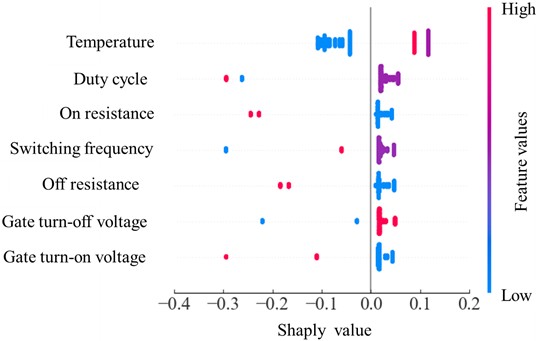
To further quantify the differences in threshold voltage degradation under various operating conditions, the daily degradation amount for each sample was extracted, as shown in Fig. 3. It can be observed that the degradation degree is relatively large in the initial stage and exhibits a monotonic decreasing trend with time overall, which is consistent with a trap-dominated degradation mechanism: in the early stress phase, rapid filling of pre-existing traps at the oxide layer and interface causes a significant threshold voltage shift, while as stress time increases, the available traps become gradually occupied, leading to a reduced capture rate and a saturating degradation trend. Based on random forest and SHAP analysis [30], as illustrated in Fig. 4, temperature, duty cycle, and on-resistance are identified as the main factors affecting degradation under various operating conditions. The mechanistic analysis based on the data provides a solid physical basis for subsequent reliability evaluation modeling.

Fig. 3Differences of the SiC MOSFET threshold voltage performance under multiple operating conditions

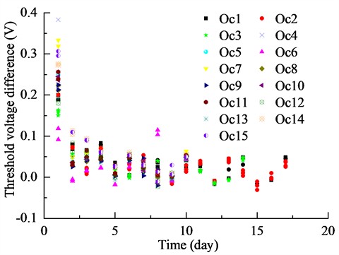
Fig. 4Analysis on influencing factors of the SiC MOSFET threshold voltage performance

5. SiC MOSFET performance degradation reliability evaluation

5.1. Flowchart of reliability evaluation

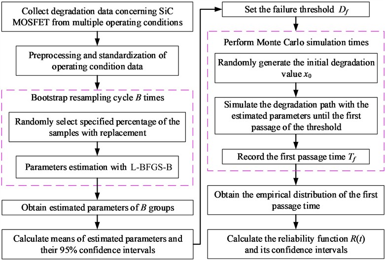
The reliability evaluation flowchart for SiC MOSFET under multiple conditions based on the nonlinear Wiener process is shown in Fig. 5, and the steps are as follows:

(1) Organize the threshold voltage degradation data of SiC MOSFET under various operating conditions, and normalize the influencing factors in each operating condition to ensure the scale consistency of each influencing factor during the modeling process.

(2) Establish a nonlinear Wiener process model and specify the parameters to be estimated in the model, including: the distribution parameters $μ_{0}$ and $σ_{0}$ of the initial values $x_{0}$ ; coefficient of influencing factors $β = [β_{0}, β_{1}, \dots β_{C}]$ ; the power exponent of time $γ$ and the diffusion coefficient $σ$ – a total of 12 parameters to be estimated.

(3) The uncertainty of the parameters to be estimated is quantified using the Bootstrap method. By randomly selecting specified percentage of the samples with replacement, model parameter estimation is achieved based on Eqs. (12) and (13). This random sampling process is repeated 50 times, and probability statistics are conducted on each set of estimated parameters. Finally, the confidence intervals for each parameter are obtained based on Eq. (14).

(4) Set the failure threshold and the total number of simulations. At each simulation, the initial value $x_{0}$ is randomly generate, and the first passage time is recorded. Finally, the reliability and its confidence intervals are calculated according to Eq. (16).

Fig. 5Flowchart of SiC MOSFET reliability evaluation

5.2. Reliability analysis

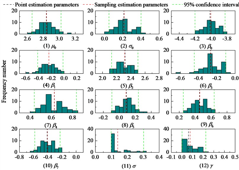
The estimated parameters are shown in Table 2, including the point estimation based on the L-BFGS-B of the 35 samples, and the Bootstrap estimation with their 95 % confidence intervals with sampling proportions of 70 %, 80 %, and 90 %, respectively. It can be seen that the relative errors between point estimation and sampling estimation with the proportion of 70 % are relatively small, as shown in Fig. 6, and all are controlled within a 95 % confidence interval. Due to inconsistent sample sizes under different operating conditions, some operating conditions are not represented during sampling, leading to significant fluctuations in the estimated parameters, especially $γ$ and $σ$ . Here, $γ$ lies at the constraint boundary, indicating that the actual optimal solution may be less than 0.1, although numerical stability constraints need to be considered during the solution process. Considering the computation efficiency and accuracy, the sampling proportion of 70 % is selected.

Excluding the uncertainty introduced by the random diffusion term $σ B (t)$ in the prediction process, the model fitting effect is evaluated using the estimation parameters obtained from all samples. The selected indicators are as follows:

Root mean square error (RMSE):

17

R M S E = \sqrt{\frac{1}{n} \sum_{i = 1}^{n} {(y_{i} - {\hat{y}}_{i})}^{2}} .

Table 2Parameter estimation

Parameters	L-BFGS-B	Bootstrap and the 95 % confidence interval
Parameters	L-BFGS-B	70 %	80 %	90 %
$μ_{0}$	2.8372	2.8389 [2.6413, 2.9911]	2.8394 [2.6737, 3.0256]	2.8007 [2.6785, 2.9925]
$σ_{0}$	0.2115	0.1712 [0.0613, 0.3887]	0.1943 [0.0477, 0.4654]	0.1377 [0.0686, 0.4137]
$β_{0}$	–4.0140	–3.9670 [–4.1937, –3.8056]	–4.0383 [–4.2175, –3.8631]	–3.9315 [–4.2731, –3.8272]
$β_{1}$	–0.2383	–0.2241 [–0.4541, –0.0468]	–0.2158 [–0.4066, –0.0541]	–0.2369 [–0.3932, –0.0757]
$β_{2}$	2.3206	2.1898 [2.1813, 2.5256]	2.3162 [2.1628, 2.4757]	2.3754 [2.1188, 2.5600]
$β_{3}$	–0.2689	–0.3457 [–0.4675, –0.0929]	–0.3228 [–0.4509, –0.1382]	–0.3957 [–0.4429, –0.1036]
$β_{4}$	0.6294	0.7037 [0.5013, 0.9043]	0.5308 [0.4477, 0.7867]	0.5314 [0.4835, 0.7942]
$β_{5}$	0.0895	0.0689 [–0.1204, 0.3011]	0.2235 [–0.0993, 0.2424]	0.1401 [–0.0618, 0.3148]
$β_{6}$	0.4533	0.4610 [0.2818, 0.6493]	0.4869 [0.2538, 0.6477]	0.3572 [0.2667, 0.6463]
$β_{7}$	–0.4092	–0.4032 [–0.5827, –0.2235]	–0.2791 [–0.6525, –0.2191]	–0.3005 [–0.5880, –0.2174]
$γ$	0.1000	0.1491 [0.1000, 0.2428]	0.2193 [0.1000, 0.2747]	0.1198 [0.1000, 0.2619]
$σ$	0.0626	0.1891 [0.0010, 0.2367]	0.2589 [0.0010, 0.2634]	0.0010 [0.0010, 0.2529]

Fig. 6Uncertainty of the evaluated parameters

Goodness of fit:

18

R^{2} = 1 - \frac{\sum_{i = 1}^{n} {(y_{i} - {\hat{y}}_{i})}^{2}}{\sum_{i = 1}^{n} {(y_{i} - {\bar{y}}_{i})}^{2}},

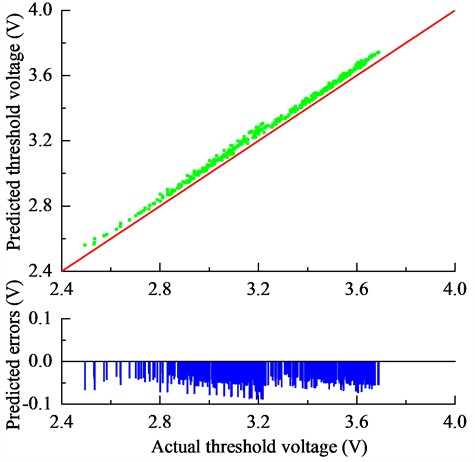
where $n$ is the number of predicted samples; $y_{i}$ and ${\hat{y}}_{i}$ are the actual threshold voltage and the predicted threshold voltage respectively, and ${\bar{y}}_{i}$ is the mean of the actual threshold voltage. The goodness of fit $R^{2}$ is within the range of 0 to 1, and the closer its value approaches 1, the stronger the explanatory power of the model on the data. After calculation, the RMSE of the nonlinear Wiener process model is 0.0458, and the goodness of fit is 0.9728. The threshold voltage predicted based on the nonlinear Wiener process model is shown in Fig. 7, as well as the error compared to the actual threshold voltage. The error is equal to the actual threshold voltage minus the predicted threshold voltage. Since the predicted threshold voltage values are mostly larger than the actual values throughout the degradation process, the predicted degradation trajectory is upper-bounded relative to the actual trajectory. Under the assumption of monotonic degradation and an upper failure threshold, this results in earlier predicted failure times at the mean level, thereby yielding a conservative estimate of the mean reliability. However, it should be noted that conservativeness at the distribution level (e.g., confidence bounds) requires further verification.

Fig. 7Prediction of threshold voltage with errors

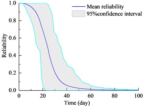
A working condition is designed with gate turn-on voltage 20 V, gate turn-off voltage -5 V, duty cycle 50 %, switching frequency 50 kHz, on resistance 10 R, off resistance 10R, temperature 25 ℃. Based on this model, 10000 simulations of the performance degradation paths of SiC MOSFET were conducted, as illustrated in Fig. 8. The failure threshold $D_{f}$ was set as 4 V to obtain the first passage time distribution. Under the sampling proportions of 70 %, 80 %, and 90 %, the mean lifetime of the SiC MOSFET respectively are 24.88, 25.98 and 26.34 days. With 200 repetitions of each group parameters estimated based on the Bootstrap method under the sampling proportions of 70 %, the reliability function curve and its 95 % confidence interval obtained through Monte Carlo simulation under designed conditions is shown in Fig. 9. It could be seen that the reliability decreases monotonically with time, which is consistent with the cumulative nature of threshold voltage degradation. Notably, the width of the 95 % confidence interval exhibits a time-dependent pattern: it is relatively wide in the early stage, narrows during the mid-life period, and widens again as the failure threshold is approached. This shape can be interpreted from both statistical and physical perspectives. The early-stage width reflects the combined effect of initial-value randomness among individual devices and parameter estimation uncertainty under small-sample conditions-both of which contribute to greater dispersion in predicted lifetimes during the initial phase. The subsequent narrowing indicates that the degradation paths converge as devices enter the stable degradation stage, where the deterministic drift component dominates and the relative influence of initial variability diminishes. The final widening near the failure threshold arises from the inherent variability in first passage time: small differences in degradation rate lead to significantly different failure times when the degradation trajectory approaches the threshold, a phenomenon commonly observed in wear-out failures.

Fig. 8Simulation degradation path and failure time distribution

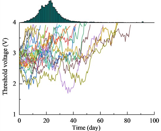
Fig. 9Reliability evaluation under the specified conditions

6. Conclusions

An efficient method based on the nonlinear Wiener process is proposed for SiC MOSFET reliability evaluation with threshold voltage degradation data of small samples under multiple operating conditions. The main conclusions and innovations are as follows:

1) The main effect factors of threshold voltage degradation in SiC MOSFET are revealed. Through random forest and SHAP analysis, it is found that temperature, duty cycle, and on resistance are the top three key factors affecting degradation rate, providing quantitative basis for the optimization of SiC MOSFET operating conditions and accelerated test design.

2) By decomposing the drift coefficient into a time-dependent nonlinear term and an operating condition influence term, the parameters corresponding to the two physical effects are separated, allowing for independent analysis of the influences of environmental factors and material aging mechanisms on the degradation rate, thereby enhancing the physical interpretability of the model.

3) An uncertainty quantification framework for reliability evaluation under small sample conditions has been proposed. By combining Bootstrap resampling with Monte Carlo simulation, a 95 % confidence interval for the reliability curve was obtained with 35 samples.

This study provides a new method for reliability evaluation of power semiconductor devices that balances accuracy and interpretability, which can be directly applied to life prediction and health management of SiC MOSFETs. Subsequent research will explore modeling of multi-stress coupling effects and achieve real-time reliability updates by combining online monitoring data.

References

L. Stevanovic et al., “High performance SiC MOSFET module for industrial applications,” in 28th International Symposium on Power Semiconductor Devices and ICs (ISPSD), pp. 479–482, Jun. 2016, https://doi.org/10.1109/ispsd.2016.7520882

Publisher
B. Shi et al., “A review of silicon carbide MOSFETs in electrified vehicles: Application, challenges, and future development,” IET Power Electronics, Vol. 16, No. 12, pp. 2103–2120, May 2023, https://doi.org/10.1049/pel2.12524

Publisher
B. J. Nel and S. Perinpanayagam, “A brief overview of SiC MOSFET failure modes and design reliability,” Procedia CIRP, Vol. 59, pp. 280–285, Jan. 2017, https://doi.org/10.1016/j.procir.2016.09.025

Publisher
G. Akbar, A. Di Fatta, G. Rizzo, G. Ala, P. Romano, and A. Imburgia, “Comprehensive review of wide-bandgap (WBG) devices: SiC MOSFET and its failure modes affecting reliability,” Physchem, Vol. 5, No. 1, Mar. 2025, https://doi.org/10.3390/physchem5010010

Publisher
H. Jiang et al., “A physical explanation of threshold voltage drift of SiC MOSFET induced by gate switching,” IEEE Transactions on Power Electronics, Vol. 37, No. 8, pp. 8830–8834, Aug. 2022, https://doi.org/10.1109/tpel.2022.3161678

Publisher
D. Xie et al., “Threshold voltage hysteresis investigation of SiC MOSFETs with different structures under various measurement conditions,” Microelectronics Reliability, Vol. 168, p. 115657, May 2025, https://doi.org/10.1016/j.microrel.2025.115657

Publisher
J. Zhang et al., “A review of reliability assessment and lifetime prediction methods for electrical machine insulation under thermal aging,” Energies, Vol. 18, No. 3, p. 576, Jan. 2025, https://doi.org/10.3390/en18030576

Publisher
H. Wang and F. Blaabjerg, “Power electronics reliability: state of the art and outlook,” IEEE Journal of Emerging and Selected Topics in Power Electronics, Vol. 9, No. 6, pp. 6476–6493, Dec. 2021, https://doi.org/10.1109/jestpe.2020.3037161

Publisher
A. Safari, A. Oshnoei, and F. Blaabjerg, “A review of recent AI applications in next-generation power electronics,” Applied Energy, Vol. 402, p. 126923, Dec. 2025, https://doi.org/10.1016/j.apenergy.2025.126923

Publisher
N. Gorjian, L. Ma, M. Mittinty, P. Yarlagadda, and Y. Sun, “A review on degradation models in reliability analysis,” in Engineering asset lifecycle management, London: Springer London, 2010, pp. 369–384, https://doi.org/10.1007/978-0-85729-320-6_42

Publisher
A. F. Shahraki, “A review on degradation modelling and its engineering applications,” International Journal of Performability Engineering, Vol. 13, No. 3, pp. 299–314, Jan. 2017, https://doi.org/10.23940/ijpe.17.03.p6.299314

Publisher
S. Li, Z. Chen, Q. Liu, W. Shi, and K. Li, “Modeling and analysis of performance degradation data for reliability assessment: a review,” IEEE Access, Vol. 8, pp. 74648–74678, Jan. 2020, https://doi.org/10.1109/access.2020.2987332

Publisher
C. J. Lu and W. O. Meeker, “Using degradation measures to estimate a time-to-failure distribution,” Technometrics, Vol. 35, No. 2, pp. 161–174, Mar. 2012, https://doi.org/10.1080/00401706.1993.10485038

Publisher
J. S. Wang, Y. Z. He, Y. D. Wang, and W. H. Liu, “Statistical analysis of the degradation data based on pseudo-life distribution,” Advanced Materials Research, Vol. 933, pp. 784–788, May 2014, https://doi.org/10.4028/www.scientific.net/amr.933.784

Publisher
J. Zhang, Y. Zhao, M. Liu, and L. Kong, “A Tukey’s g-and-h distribution based approach with PSO for degradation reliability modeling,” Engineering Computations, Vol. 36, No. 5, pp. 1699–1715, Jun. 2019, https://doi.org/10.1108/ec-11-2017-0428

Publisher
L. Liu, X. Li, F. Sun, and N. Wang, “A general accelerated degradation model based on the Wiener Process,” Materials, Vol. 9, No. 12, p. 981, Dec. 2016, https://doi.org/10.3390/ma9120981

Publisher
M. Giorgio, A. Piscopo, and G. Pulcini, “A new Wiener process with bathtub-shaped degradation rate in the presence of random effects,” Applied Stochastic Models in Business and Industry, Vol. 40, No. 3, pp. 574–597, May 2023, https://doi.org/10.1002/asmb.2749

Publisher
L. A. Rodríguez-Picón, L. C. Méndez-González, V. H. Flores-Ochoa, I. J. Pérez Olguín, and V. García, “Degradation modeling based on the gamma process with random initial degradation level and random threshold,” Quality Technology and Quantitative Management, Vol. 20, No. 6, pp. 730–750, Jun. 2023, https://doi.org/10.1080/16843703.2022.2146904

Publisher
Z. Zhang et al., “A reliability evaluation method for gamma processes with multiple random effects,” Machines, Vol. 11, No. 9, p. 905, Sep. 2023, https://doi.org/10.3390/machines11090905

Publisher
T. Santini et al., “Accelerated degradation data of SiC MOSFETs for lifetime and remaining useful life assessment,” Microelectronics Reliability, Vol. 54, No. 9-10, pp. 1718–1723, Sep. 2014, https://doi.org/10.1016/j.microrel.2014.07.082

Publisher
H. Zheng, J. Yang, W. Kang, and Y. Zhao, “Accelerated degradation data analysis based on inverse Gaussian process with unit heterogeneity,” Applied Mathematical Modelling, Vol. 126, pp. 420–438, Feb. 2024, https://doi.org/10.1016/j.apm.2023.11.003

Publisher
K. Yang and Y. Qi, “Accelerated degradation reliability modeling based on multiple uncertainty Wiener Processes,” International Journal of Mechanical and Electrical Engineering, Vol. 1, No. 1, pp. 109–118, Dec. 2023, https://doi.org/10.62051/ijmee.v1n1.12

Publisher
D. Pan, S. Lu, Y. Liu, W. Yang, and J.-B. Liu, “Degradation data analysis using a Wiener degradation model with three-source uncertainties,” IEEE Access, Vol. 7, pp. 37896–37907, Jan. 2019, https://doi.org/10.1109/access.2019.2906325

Publisher
J. Li, Z. Wang, X. Liu, Y. Zhang, H. Fu, and C. Liu, “A Wiener process model for accelerated degradation analysis considering measurement errors,” Microelectronics Reliability, Vol. 65, pp. 8–15, Oct. 2016, https://doi.org/10.1016/j.microrel.2016.08.004

Publisher
Q. Zhai, P. Chen, L. Hong, and L. Shen, “A random-effects Wiener degradation model based on accelerated failure time,” Reliability Engineering and System Safety, Vol. 180, pp. 94–103, Dec. 2018, https://doi.org/10.1016/j.ress.2018.07.003

Publisher
L. Sun, F. Zhao, N. Balakrishnan, H. Zhou, and X. Gu, “A nonlinear Wiener degradation model integrating degradation data under accelerated stresses and real operating environment,” Proceedings of the Institution of Mechanical Engineers, Part O: Journal of Risk and Reliability, Vol. 235, No. 3, pp. 356–373, Dec. 2020, https://doi.org/10.1177/1748006x20978099

Publisher
Q. Huang, J. Tang, and X. Feng, “Reliability assessment model for multiple stress factors accelerated degradation test using a Wiener process with random effects,” PLOS One, Vol. 20, No. 6, p. e0325117, Jun. 2025, https://doi.org/10.1371/journal.pone.0325117

Publisher
K. Puschkarsky, T. Grasser, T. Aichinger, W. Gustin, and H. Reisinger, “Review on SiC MOSFETs high-voltage device reliability focusing on threshold voltage instability,” IEEE Transactions on Electron Devices, Vol. 66, No. 11, pp. 4604–4616, Nov. 2019, https://doi.org/10.1109/ted.2019.2938262

Publisher
Q. Wu, B. Xu, L. Xiao, and Q. Wang, “A remaining useful life prediction method of SiC MOSFET considering failure threshold uncertainty,” IET Power Electronics, Vol. 17, No. 12, pp. 1594–1606, Nov. 2023, https://doi.org/10.1049/pel2.12611

Publisher
Y. Kim and Y. Kim, “Explainable heat-related mortality with random forest and SHapley Additive exPlanations (SHAP) models,” Sustainable Cities and Society, Vol. 79, p. 103677, Apr. 2022, https://doi.org/10.1016/j.scs.2022.103677

Publisher

About this article

Received

November 2, 2025

Accepted

May 2, 2026

Published

June 4, 2026

DOI

https://doi.org/10.21595/jme.2026.25806

Keywords

SiC MOSFET

nonlinear wiener process

multiple conditions

threshold voltage

performance degradation

reliability evaluation

Acknowledgements

The authors have not disclosed any funding.

Data Availability

The datasets generated during and/or analyzed during the current study are available from the corresponding author on reasonable request.

Author Contributions

Yaoheng Li: writing-original draft preparation, test design and validation. Jinbao Zhang: supervision and conceptualization. Hui Wang: writing-review and editing. Jinle Zhang: software. Haiquan Zhang: bench test. Fuqiang Zhao: bench test.

Conflict of interest

The authors declare that they have no conflict of interest.

This is an open access article distributed under the Creative Commons Attribution License, which permits unrestricted use, distribution, and reproduction in any medium, provided the original work is properly cited.

Y. Li, J. Zhang, H. Wang, J. Zhang, H. Zhang, and F. Zhao, “Reliability evaluation of SiC MOSFET with performance degradation under multiple conditions based on nonlinear wiener process,” Journal of Measurements in Engineering, Vol. 14, No. 3, –13, Jun. 2026, https://doi.org/10.21595/jme.2026.25806

Copy Extrica

Copied to clipboard!

TY  - JOUR
DO  - 10.21595/jme.2026.25806
UR  - https://doi.org/10.21595/jme.2026.25806
TI  - Reliability evaluation of SiC MOSFET with performance degradation under multiple conditions based on nonlinear wiener process
T2  - Journal of Measurements in Engineering
AU  - Li, Yaoheng
AU  - Zhang, Jinbao
AU  - Wang, Hui
AU  - Zhang, Jinle
AU  - Zhang, Haiquan
AU  - Zhao, Fuqiang
PY  - 2026
DA  - 2026/06/04
PB  - Extrica
VL  - 14
IS  - 3
SN  - 2335-2124
SN  - 2424-4635
ER  - 

Copy Ris

Copied to clipboard!

@article{doi_10.21595/jme.2026.25806,
  title = {Reliability evaluation of SiC MOSFET with performance degradation under multiple conditions based on nonlinear wiener process},
  author = {Li, Yaoheng and Zhang, Jinbao and Wang, Hui and Zhang, Jinle and Zhang, Haiquan and Zhao, Fuqiang},
  journal = {Journal of Measurements in Engineering},
  year = {2026},
  month = {6},
  volume = {14},
  number = {3},
  doi = {10.21595/jme.2026.25806},
  url = {https://doi.org/10.21595/jme.2026.25806},
  publisher = {Extrica},
  issn = {2335-2124},
  eissn = {2424-4635},
}

Copy Bibtex

Copied to clipboard!

[1]Y. Li, J. Zhang, H. Wang, J. Zhang, H. Zhang, and F. Zhao, “Reliability evaluation of SiC MOSFET with performance degradation under multiple conditions based on nonlinear wiener process,” Journal of Measurements in Engineering, Jun. 2026, doi: 10.21595/jme.2026.25806.

Copy IEEE

Copied to clipboard!

Li, Yaoheng, Jinbao Zhang, Hui Wang, Jinle Zhang, Haiquan Zhang, and Fuqiang Zhao. “Reliability evaluation of SiC MOSFET with performance degradation under multiple conditions based on nonlinear wiener process.” Journal of Measurements in Engineering 14, no. 3 (2026). https://doi.org/10.21595/jme.2026.25806.

Copy Chicago

Copied to clipboard!