Abstract
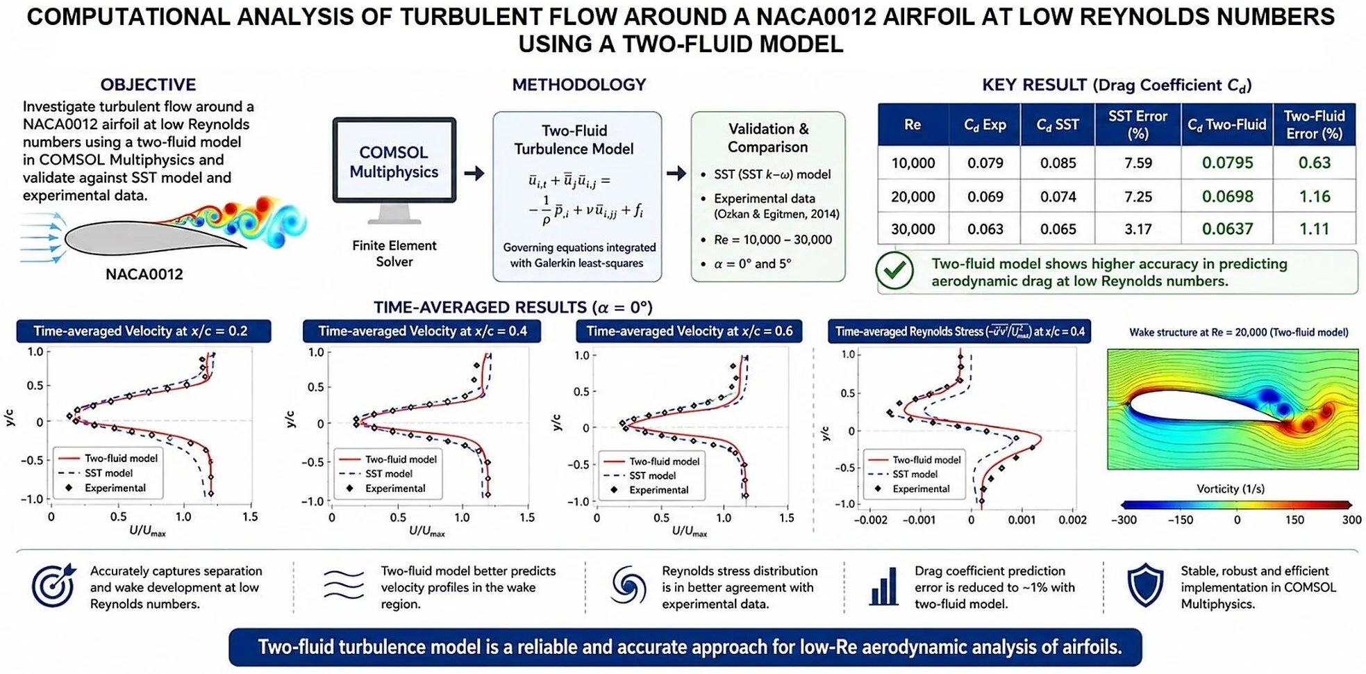
This paper presents a detailed numerical investigation of the turbulent flow structure around a NACA0012 airfoil at low Reynolds numbers using a two-fluid turbulence model implemented in the COMSOL Multiphysics environment. The study focuses on Reynolds numbers ranging from 10,000 to 30,000 at an angle of attack of 0°, and from 10,000 to 25,000 at 5°. The primary objective is to assess the capability of the two-fluid model in accurately capturing the flow separation, wake development, and turbulent stress distribution in the low-Reynolds-number regime. The obtained numerical results are systematically compared with those from the widely used Menter’s SST (Shear Stress Transport) model and available experimental data from literature to validate the accuracy and robustness of the proposed approach. The simulations demonstrate that the two-fluid turbulence model provides improved agreement with experimental measurements, particularly in predicting the velocity profiles and Reynolds stress distributions in the near-wake region. The implementation of the model within the COMSOL Multiphysics framework shows high numerical stability, reliable convergence, and computational efficiency across all tested flow regimes. Furthermore, the two-fluid model exhibits enhanced capability in describing complex anisotropic turbulence effects that are often underrepresented in traditional RANS-based models. The outcomes of this study confirm that the two-fluid turbulence model is a promising and accurate alternative for analyzing low-Reynolds-number aerodynamics, offering valuable insights for the design and optimization of small-scale air vehicles, micro air vehicles (MAVs), and other low-speed aerodynamic systems.
Highlights
- Local mesh refinement significantly improves the prediction of shock-wave behavior in transonic flow over the RAE 2822 airfoil.
- The refined mesh provides a sharper resolution of strong Mach number, velocity, pressure, temperature, and density gradients in the shock region.
- The two-fluid approach effectively captures flow separation, wake development, and anisotropic turbulent structures at Reynolds numbers from 10,000 to 30,000.
- Numerical results demonstrate reliable performance of the two-fluid model at angles of attack of 0∘ and 5∘.
- Grid-independence analysis confirms that approximately 81,200 computational elements provide sufficient numerical accuracy at reasonable computational cost.
1. Introduction
The NACA0012 airfoil is one of the most common airfoils for airplane and other aircraft wings. It has a thickness of 12 % of the chord and a symmetrical shape, making it ideal for use on wings that must generate lift both up and down.
At low Reynolds numbers, i.e. At low air velocities, the NACA0012 airfoil behaves somewhat differently than at higher air velocities. In particular, at low Reynolds numbers, there is an increase in drag and a deterioration in the aerodynamic characteristics of the airfoil.
At low Reynolds numbers, i.e. At low air velocities, the NACA0012 airfoil can show unexpected properties, such as separation of the air flow from the airfoil surface and the occurrence of turbulence.
In this case, the wake behind the profile can be unstable and non-linear, with changes in the direction and speed of the air flow at different points in the profile. In addition, vortex structures and areas of increased resistance can occur, which can lead to loss of controllability and stability of the aircraft.
Commercial aviation has long been a primary focus of aerodynamic research, with much attention focused on high Reynolds number flows, as measured by chord length (Rec > 500,000). However, in recent decades, interest in low Reynolds number flows (10,000 < Rec < 100,000) has increased significantly due to their key role in the design and development of small unmanned aerial vehicles (UAVs). This category includes micro- (MAVs) and nano- (NAVs), which are being actively developed for monitoring, surveillance, and remote sensing applications [1].
Experimental studies of the NACA0012 airfoil by Wang et al. [2] showed that flow regimes at Rec < 10,000 and 10,000 < Rec < 30,000 can be classified as ultra-low Reynolds number and low Reynolds number regimes, respectively. Flow visualization results indicate that in the range from ultra-low to low Rec values, the flow structure is characterized by a sequence of transition, separation, and reattachment of the boundary layer, which significantly influences the formation of the airfoil wake. The combination of these processes leads to the formation of a laminar separation bubble (LSB), which is the reattachment of the flow after laminar separation due to turbulent mixing [3].
Since the presence of a laminar separation bubble negatively impacts airfoil aerodynamic performance, most research has focused on the mechanisms behind its formation and methods for controlling this phenomenon. However, Carmichael [4] and Gad-el-Haq [3] formulated a general rule according to which the formation of a laminar separation bubble is only possible for Rec > 50,000. Therefore, in the range of 10,000 < Rec < 50,000, the airfoil typically experiences laminar separation without subsequent flow reattachment. This atypical flow behavior is accompanied by sharp changes in the lift coefficient when transitioning from ultra-low to low Reynolds numbers [5], especially under conditions of developed flow separation.
Similar conclusions are presented in the work of Alam et al. [6], who analyzed the main flow characteristics at various angles of attack and demonstrated an increase in the lift coefficient over a wide range of Reynolds numbers – from Rec = 5300 to 360,000 [7]. Therefore, it can be argued that further research into the physics of flow around an airfoil and its wake in the range of 10,000 < Rec < 50,000 is necessary for a deeper understanding of complex flow mechanisms and the development of improved airfoil shapes for relevant engineering applications [8-11].
For mathematical modeling of the NACA0012 airfoil at low Reynolds numbers, the CFD (Computational Fluid Dynamics) computer simulation method can be used. CFD allows you to solve the Navier-Stokes equations that describe the movement of a fluid or gas inside a profile, and obtain data on pressure distribution, flow velocity and other parameters. To simulate the airfoil of NACA0012, you can use special programs such as ANSYS Fluent, OpenFOAM, STAR-CCM+, Comsol Multiphysics, etc. [12-14].
In recent decades, significant progress has been made in the development of high-precision numerical methods for solving the Navier-Stokes equations, which are used to model turbulent flows of practical significance. Computational approaches such as large-eddy simulation (LES) and direct numerical modeling (DNS) are currently being increasingly used to analyze turbulent flows. However, their practical application remains significantly limited by the high requirements for the spatiotemporal resolution of computational grids and, consequently, the significant computational costs. Therefore, the widespread adoption of these methods is directly linked to the further development of computing technology and, according to experts, is only possible in the distant future.
Therefore, for the foreseeable future, semi-empirical approaches will remain the primary tool for solving applied aerodynamic problems. Most of the semi-empirical turbulence models used are based on the Reynolds-averaged Navier-Stokes (RANS) equations. When the initial hydrodynamic equations are time-averaged, additional terms in the form of Reynolds stresses arise, requiring modeling, rendering the system of equations incomplete. To close it, numerous different mathematical models have been developed, based on the fundamental hypotheses of Boussinesq [15], Kolmogorov [16], Prandtl [17], Karman [18], and other researchers.
A comparative analysis of semi-empirical turbulence models presented in the NASA turbulence modeling database shows that the Spalart-Almaras model [19] and the Menter - SST model [20-21] demonstrate the greatest practical effectiveness. These models are currently widely used for numerical studies and solutions to a large number of relevant engineering and aerodynamic problems [22-27].
In recent years, the two-fluid turbulence model has become increasingly widespread [28-29]. This approach is based on describing the dynamics of two interacting fluids and, unlike the classical Reynolds concept, results in a closed system of equations. A significant advantage of the two-fluid model is its ability to adequately describe complex anisotropic turbulent flow structures. The problem under consideration is of great importance for aviation and rocket and space technology.
For example, in [28], a two-fluid model was applied to study flow past a flat plate, using a simplified parabolic system of equations in which the pressure was assumed to be constant and longitudinal diffusion terms were ignored. However, such assumptions are not universal, since in many engineering applications, flow develops in confined regions and is accompanied by significant pressure gradients. In [30], a two-fluid turbulence model was used to solve the problem of flow past a square within the framework of a complete system of equations, and the numerical results obtained were compared with experimental data. The description of the problem under consideration is presented in the NACA turbulence modeling database [31], where the flow over the NACA0012 airfoil at Reynolds numbers between 10,000 and 30,000 has been extensively studied using conventional turbulence models.
In this paper, this problem is considered using a two-fluid turbulence model, which differs in concept from the classical formulations of the Reynolds-averaged Navier-Stokes (RANS) equations. The two-fluid model is implemented in the COMSOL Multiphysics software environment for numerical simulation of incompressible turbulent flow around a NACA0012 airfoil at various angles of attack. It should be noted that the aerodynamic characteristics of the NACA0012 airfoil in the Reynolds number range of 10,000-30,000 have been well studied in scientific literature. Therefore, the primary objective of this study is not to develop a new theoretical turbulence model, but to numerically implement and test the applicability of the two-fluid model to external aerodynamic problems at low Reynolds numbers. The main contribution of this work lies in the implementation of a two-fluid turbulence model in COMSOL Multiphysics, as well as its verification and comparative analysis with the widely used SST turbulence model and available experimental data. This comparison allows us to evaluate the ability of the two-fluid model to reproduce the wake structure, velocity distribution, and turbulent stress under low Reynolds number conditions. Unlike traditional single-fluid turbulence models, the two-fluid approach treats turbulence as the interaction of two interpenetrating continua, allowing for a more detailed consideration of the anisotropic properties of turbulent structures and the mechanisms of momentum transfer in the flow. Implementation of the model in COMSOL Multiphysics provides a flexible numerical platform for studying flow separation processes, wake formation, and transient flow regimes. The results obtained expand the possibilities of using the two-fluid turbulence model for external aerodynamic problems and can be useful in analyzing and optimizing the aerodynamic characteristics of low-speed aircraft, micro-aircraft (MAV), and other engineering systems operating in the low Reynolds number range. The novelty of this study lies in the implementation and validation of a two-fluid turbulence model for low-Reynolds-number flow around a NACA0012 airfoil using COMSOL Multiphysics. Unlike traditional RANS models, the proposed approach provides improved prediction of wake structures and turbulent stresses, especially in transitional flow regimes.
2. Physical and mathematical formulation of the problem
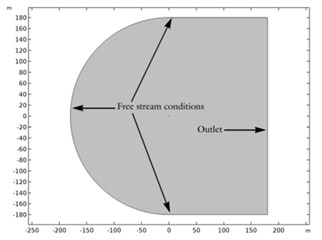
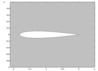
This paper examines two-dimensional turbulent flow around the symmetrical NACA 0012 airfoil, which is widely used as a reference object in the study of low-Reynolds number aerodynamic flows. The analysis is performed under the assumption of a plane flow, which allows for a detailed study of key flow structure features, such as boundary layer development, separation processes, and wake formation. The physical picture of the flow under study, as well as the geometric parameters of the airfoil and the configuration of the computational domains used for the numerical simulation, are clearly presented in Figure 1. These diagrams illustrate the location of the computational domain relative to the airfoil, as well as the main boundary conditions adopted in the problem formulation.
For the NACA 0012 airfoil problem, the Reynolds number based on the chord length is 10000 < Rec < 30000. The length of the chord 1 m. Two options for the angle of attack of the airfoil 0 and 5° are considered. The computational domain was chosen sufficiently large to eliminate the influence of far-field boundaries on the solution. The outer boundaries of the domain were located at a distance of approximately 180 chord lengths (180) from the airfoil in all directions. Such a large domain ensures negligible blockage effects and allows the wake and surrounding flow structures to develop without artificial confinement.
The boundary conditions used in the present numerical simulations are defined as follows. At the inlet boundary, a uniform velocity profile was prescribed corresponding to the selected Reynolds number. The transverse velocity component was set to zero, while the pressure was initialized with a reference value. At the outlet boundary, a zero-gradient condition for velocity was imposed together with a fixed reference pressure condition. On the airfoil surface, the no-slip boundary condition was applied for the velocity components. The perturbation velocity components associated with the two-fluid turbulence model were initialized with small values at the inlet in order to represent weak incoming disturbances in the flow field.
2.1. Mathematical model of turbulence
A two-dimensional, unsteady system of equations for a turbulent two-fluid model in Cartesian coordinates is used to mathematically describe the dynamics of turbulent flow and takes into account the interaction of two interpenetrating media. This system of equations is based on the laws of conservation of mass and momentum and allows for the modeling of both averaged flow characteristics and the specific features of turbulent pulsations. Unlike classical Reynolds approaches, the two-fluid model under consideration results in a closed system of differential equations, which significantly improves the accuracy of the description of anisotropic turbulent effects.
Equations of turbulent flow of incompressible fluid in a new two-fluid approach:
where coefficient of friction:
In this expression the largest root of the characteristic Eq. (3):
where :
In Cartesian coordinates, this unsteady system of Eqs. (1-4) can be written as follows [25]:
where:
In the above equations, , denote the streamwise and transverse components of the time-averaged flow velocity vector, respectively, while 𝑝 represents the hydrostatic pressure. The variables , correspond to the relative streamwise and transverse components of the fluid velocity. The quantities , , define the molecular kinematic viscosity components, whereas 𝜈 denotes the effective molar viscosities. The parameter 𝑑 specifies the shortest distance to the solid boundary. No additional low-Reynolds-number corrections or wall damping functions were introduced, since the two-fluid turbulence model inherently accounts for near-wall effects through the distance-to-wall parameter included in the formulation of the effective viscosities. Model constants were taken from previous validation studies of the two-fluid turbulence model and were not additionally calibrated:
Fig. 1Scheme of computational domains
а) Flow around the NACA 0012 airfoil
b) Airfoil geometry
The weak formulation of the governing equations and the transport equations of the two-fluid turbulence model follows the standard Galerkin finite element procedure implemented in COMSOL Multiphysics. The detailed derivation of the weak form of the model equations was presented in our previous work [28], and therefore is not repeated here.
The choice of the two-fluid turbulence model is motivated by its ability to represent anisotropic turbulent structures and transitional flow behavior more accurately than conventional Reynolds-averaged turbulence models. Classical RANS models, such as the SST model, rely on the Boussinesq hypothesis, which assumes isotropic turbulent viscosity and may therefore have limitations in predicting complex separated flows and transitional regimes typical for low Reynolds number aerodynamics. In contrast, the two-fluid turbulence model describes turbulence as an interaction between two interpenetrating continua representing the mean flow and fluctuating components. This formulation allows the model to capture anisotropic turbulent stresses and energy transfer mechanisms more realistically. Such effects play an important role in low-Reynolds-number flows around airfoils, where laminar separation, transition, and wake development strongly influence the aerodynamic characteristics [29].
2.2. Calculation grids
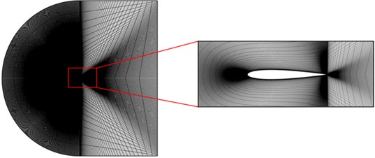
In the present study, mesh thickening near the surface of the profile in Fig. 2 was used.
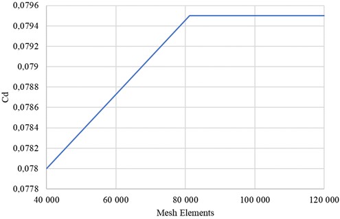
The computational mesh consisted of approximately 81,200 quadrilateral elements with 82,112 mesh vertices. The average mesh quality was 0.787, with a minimum element quality of 0.108, indicating an acceptable mesh resolution for the present simulations. The resulting finite element discretization produced a system with approximately 1.01×10⁶ degrees of freedom. For the governing system of Eq. (1), standard no-slip boundary conditions were imposed on all solid walls. At the outlet boundary, extrapolation conditions were applied for all flow variables. At the inlet, a uniform profile of the streamwise velocity component was prescribed with while the transverse velocity component and pressure were set to zero, i.e., . In addition, prescribed values of the relative (perturbation) velocity components were specified at the inlet as, , . The near-wall mesh resolution was selected such that the dimensionless wall distance remained within 1 over the entire airfoil surface. A refined boundary-layer mesh was generated near the airfoil surface in order to resolve the viscous sublayer of the boundary layer. The mesh consisted of approximately 100 elements in the wall-normal direction with an exponential growth distribution. The element expansion ratio was 1.5, which allowed gradual stretching of elements away from the wall. The viscous sublayer of the boundary layer to be directly resolved without the use of wall functions.
Fig. 2Computational mesh for flow around the profile
The graph shows the dependence of the calculated value on the number of grid elements. It is evident that as the number of elements increases from 40,000 to 80,000, there is a slight change in the drag coefficient value. With a further increase in the number of elements to 120,000, the value remains virtually unchanged, indicating that the solution achieves grid independence. Thus, the selected computational grid, containing approximately 81,200 elements, ensures sufficient accuracy of the numerical simulation at acceptable computational costs.
Fig. 3Study of the independence of the numerical solution from the computational grid size for the aerodynamic drag coefficient Cd
For comparison purposes, the standard Menter - SST turbulence model was also employed. This model combines the - formulation near the wall with the - behavior in the free stream using a blending function, providing reliable predictions for separated flows [30-31].
3. Solution method
For the numerical solution of the system of initial nonstationary Eq. (1) and for the SST turbulence model, the finite element method (FEM) was employed [32-44]. The computations were performed using the COMSOL Multiphysics 6.1 software package, which provides robust built-in solvers for solving coupled nonlinear partial differential equations governing turbulent flows. The use of the finite element approach allowed flexible discretization of the computational domain, ensuring higher spatial resolution near the airfoil surface where steep gradients in velocity and pressure occur. A non-uniform mesh with local refinement was applied in regions of high velocity and pressure gradients, particularly near the leading edge, boundary layer, and wake zone of the NACA0012 airfoil. This refinement strategy improved numerical accuracy without excessive computational cost. The time-dependent form of the governing equations was integrated using an implicit time-stepping scheme to enhance stability and convergence at low Reynolds numbers, where unsteady separation and transition phenomena are dominant. In addition, stabilization techniques inherent to the Galerkin least-squares formulation were utilized to suppress numerical oscillations arising from convection-dominated flow behavior. The convergence criteria for both velocity and pressure fields were set to 10−3, ensuring reliable and consistent solutions across all simulation cases. The iterative solvers available in COMSOL Multiphysics (based on the PARDISO and GMRES algorithms) demonstrated excellent performance for the two-fluid turbulence model, achieving rapid convergence even under complex flow conditions. Overall, the combination of the two-fluid turbulence formulation with the finite element method in the COMSOL Multiphysics environment provided an efficient and accurate computational framework for simulating low-Reynolds-number aerodynamic flows. This approach allowed for detailed analysis of wake structures, turbulent stress distributions, and pressure variations with high numerical fidelity. In the present simulations linear shape functions (P1 elements) were employed for both velocity and pressure variables. To ensure numerical stability of the equal-order interpolation, stabilization techniques inherent to the Galerkin least-squares formulation implemented in COMSOL Multiphysics were applied.
3.1. Calculation results and their discussion
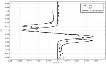
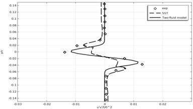
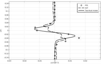
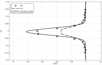
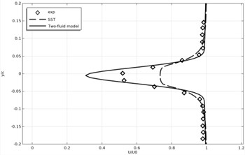
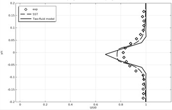
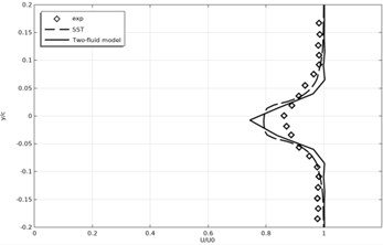
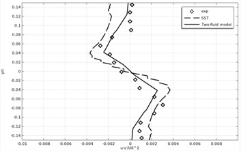
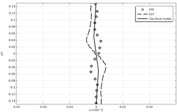
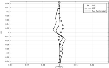
Time-averaged and normalized longitudinal velocity profiles are used to analyze flow characteristics at various downstream cross-sections of an airfoil. Profile normalization means converting the velocity values at each point to dimensionless form by dividing by the maximum velocity value in the corresponding airfoil. In this study, the time-averaged and normalized longitudinal velocity profiles were analyzed at three typical downstream cross-sections: 𝑥/𝑐 = 0.2, 0.4, and 0.6. Due to the symmetrical geometry of the NACA0012 airfoil at zero angle of attack ( 0°), the resulting velocity profiles are also symmetrical about the airfoil chord. Figs. 4-5 show the time-averaged and normalized longitudinal velocity profiles, as well as the averaged Reynolds stress values at the cross-section 𝑥/𝑐 = 0.2. The solid lines show the results obtained using the two-fluid model, the dotted lines show the data from the SST model, while the experimental results are shown as diamond-shaped markers (Ozkan G. M., Egitmen H) [7].
The experimental data used for validation were taken from the study reported in [7]. In that work, aerodynamic measurements for the NACA0012 airfoil were performed in a low-speed wind tunnel under controlled laboratory conditions. Velocity and pressure distributions were obtained using standard measurement techniques, and the reported experimental uncertainty was within the typical range for low-Reynolds-number aerodynamic experiments. These experimental results provide a reliable reference for assessing the accuracy of the numerical simulations performed in the present study.
The velocity profiles were normalized by the maximum velocity within the profile. It should be noted that normalization by the free-stream velocity may provide a clearer representation of the wake velocity deficit; however, the present normalization was adopted to facilitate comparison of the velocity distribution shapes at different locations.
Figs. 4-5 show that for the angles of attack 0°. The largest deviation from the experiment [7] for longitudinal velocity and Reynolds stress occurs at / = 1.2 at Reynolds number Rec = 30000.
Fig. 4Time-averaged velocity profiles at x/c = 0.2 for different Reynolds numbers, showing comparison between the two-fluid model, SST model, and experimental data
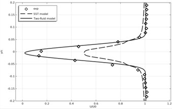
a) Re = 10000
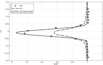
b) Re = 15000
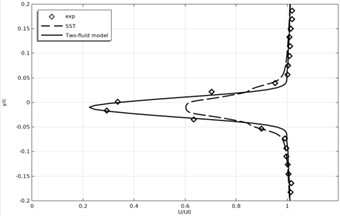
c) Re = 20000
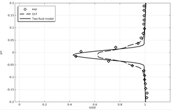
d) Re = 25000
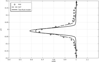
e) Re = 30000
Fig. 5Time-averaged Reynolds stress profiles
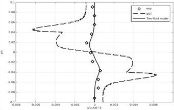
a) Re = 10000
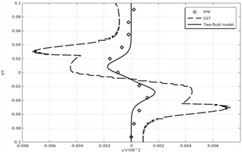
b) Re = 15000
c) Re = 20000
d) Re = 25000
e) Re = 30000
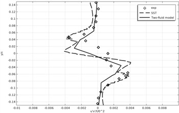
Figs. 6-7 shows the time-averaged and normalized longitudinal velocity and Reynolds stress profiles at / = 0.4.
Fig. 6Time-averaged and normalized longitudinal velocity profiles
a) Re = 10000
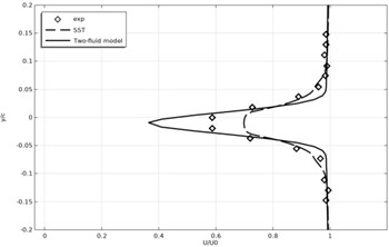
b) Re = 15000
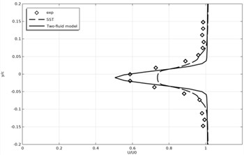
c) Re = 20000
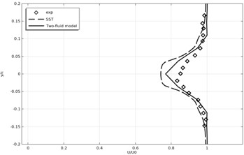
d) Re = 25000
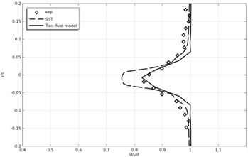
e) Re = 30000
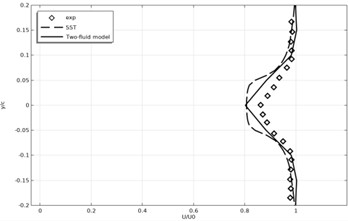
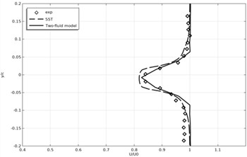
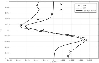
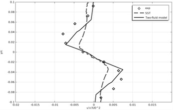
Figs. 8-9 show the time-averaged and normalized longitudinal velocity and Reynolds stress profiles at / = 0.6.
Figs. 8-9 show that the deviation of the results is already greater than in the sections / = 0.4 and / = 0.6. But in general, we can say that the results of the model are in good agreement with the experimental data.
Fig. 7Time-averaged Reynolds stress
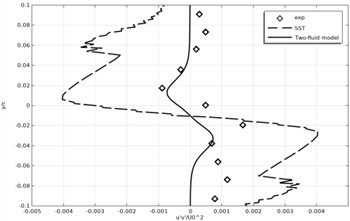
a) Re = 10000
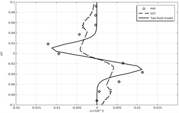
b) Re = 15000
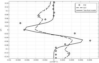
c) Re = 20000
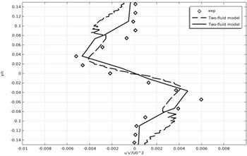
d) Re = 25000
e) Re = 30000
Fig. 8Time-averaged and normalized longitudinal velocity profiles
a) Re = 10000
b) Re = 15000
c) Re = 20000
d) Re = 25000
e) Re = 30000
Fig. 9Time-averaged Reynolds stress
a) Re = 10000
b) Re = 15000
c) Re = 20000
d) Re = 25000
e) Re = 30000
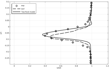
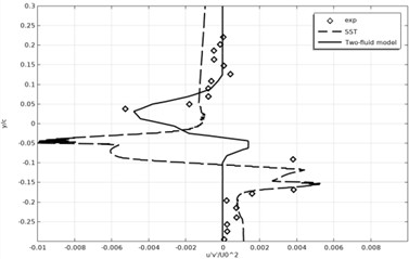
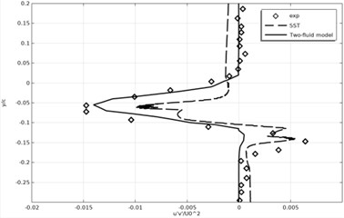
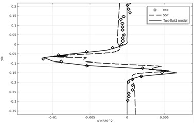
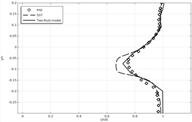
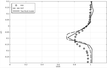
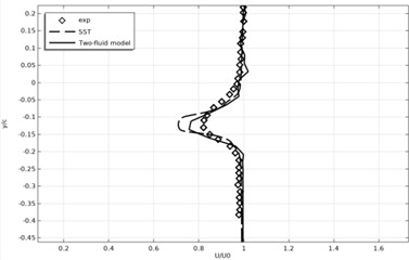
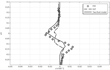
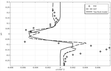
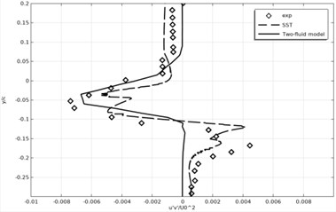
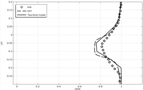
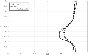
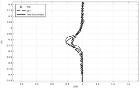
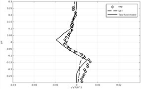
Figs. 10-11 show the time-averaged and normalized profiles of the longitudinal velocity and Reynolds stress at the point / = 0.2 at an angle of attack 5°.
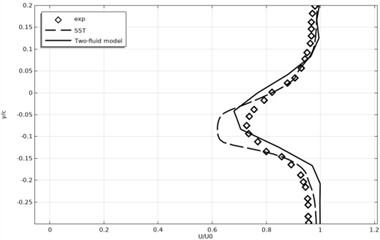
Figs. 12-13 show the time-averaged and normalized longitudinal velocity profiles and the time-averaged Reynolds stress at the point / = 0.4.
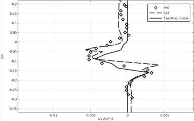
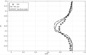
Figs. 14-15 show the time-averaged and normalized longitudinal velocity and Reynolds stress profiles at the point / = 0.6.
At the angle of attack 5°, the flow over the airfoil remains predominantly transitional. The boundary layer on the suction side experiences an adverse pressure gradient, which may lead to the formation of a laminar separation bubble. In this regime, the flow separates locally from the surface and subsequently reattaches downstream due to transition to turbulence in the separated shear layer. Such separation behavior is typical for airfoils operating at low Reynolds numbers and has a significant influence on the wake structure and aerodynamic characteristics of the flow.
Fig. 10Time-averaged and normalized longitudinal velocity profiles
a) Re = 10000
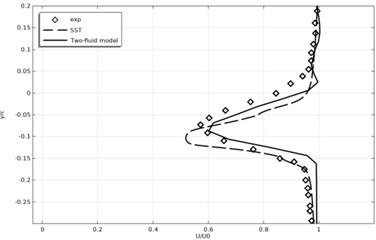
b) Re = 15000
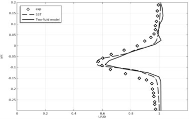
c) Re = 20000
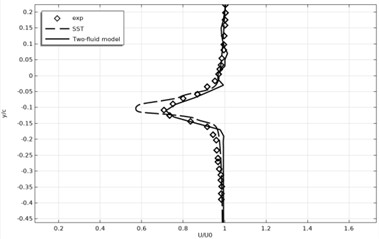
d) Re = 25000
Fig. 11Time-averaged Reynolds stress profiles
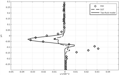
a) Re = 10000
b) Re = 15000
c) Re = 20000
d) Re = 25000
Fig. 12Time-averaged and normalized longitudinal velocity profiles
a) Re = 10000
b) Re = 15000
c) Re = 20000
d) Re = 25000
Fig. 13Time-averaged Reynolds stress profiles
a) Re = 10000
b) Re = 15000
c) Re = 20000
d) Re = 25000
The distribution of the airfoil surface pressure coefficient reflects the pattern of pressure variation along its surface as a function of distance from a selected reference point. For quantitative analysis of this distribution, the surface pressure coefficient is typically used. It is defined as a dimensionless quantity equal to the ratio of the difference between the local airfoil surface pressure and the undisturbed flow pressure to the dynamic free-flow pressure:
where, denotes the pressure at the given point on the airfoil surface, is the undisturbed free-flow pressure, is the free-flow density, and is the characteristic free-flow velocity.
Fig. 14Time-averaged and normalized longitudinal velocity profiles
a) Re = 10000
b) Re = 15000
c) Re = 20000
d) Re = 25000
Fig. 15Time-averaged Reynolds stresses
a) Re = 10000
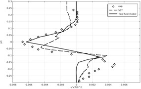
b) Re = 15000
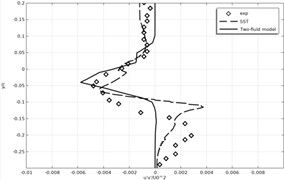
c) Re = 20000
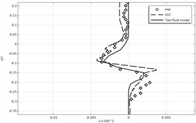
d) Re = 25000
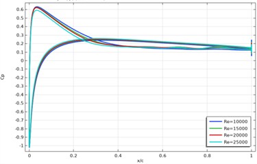
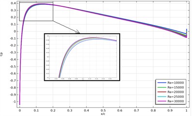
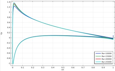
Plots of the pressure coefficient distribution typically distinguish regions of positive and negative pressure values. The positive pressure region is typically associated with the generation of lift, while the negative pressure region is associated with the generation of aerodynamic drag. Analyzing the distribution of the surface pressure coefficient along the wing airfoil allows us to evaluate its key aerodynamic characteristics, including lift, drag coefficient, and other parameters. Fig. 16 shows the distribution of the surface pressure coefficient for various angles of attack 0°, 5°.
Fig. 16Distribution of surface pressure coefficient Cp
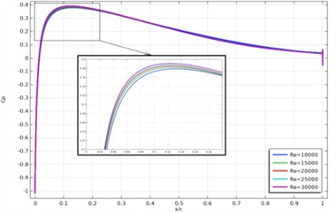
a) Two-fluid model, 0°
b) Two-fluid model, 5°
c) SST, 0°
d) SST, 5°
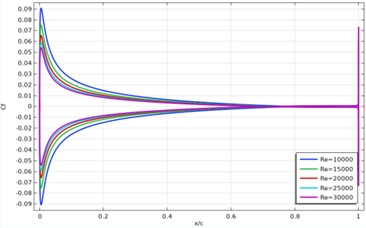
The distribution of the friction coefficient on the airfoil surface reflects the change in shear stress acting on the wing surface depending on the distance from a selected reference point. The friction coefficient is defined as a dimensionless quantity equal to the ratio of the friction force acting on the airfoil surface to the dynamic pressure of the undisturbed flow:
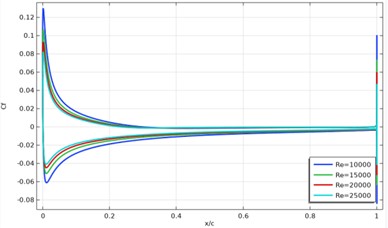
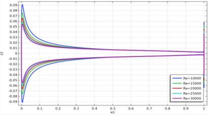
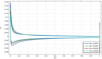
where, 𝐹 denotes the friction force acting on the airfoil surface, and 𝑆 denotes the airfoil surface area oriented along the flow direction. To study the friction coefficient distribution along a wing airfoil, plots of versus distance measured from a selected point on the surface are typically used. Analysis of such plots allows us to identify regions with higher and lower friction coefficient values. For the symmetric airfoil NACA0012 at 0°, the pressure coefficient distributions on the upper and lower surfaces are nearly identical due to flow symmetry. At 5°, the pressure distributions become asymmetric, resulting in a noticeable difference between the suction and pressure sides of the airfoil. Typically, the zone of increased friction is localized near the airfoil's leading edge and also manifests itself in the flow separation region on the upper wing surface, as clearly demonstrated in Fig. 17.
Table 1 presents a comparative analysis of the minimum aerodynamic drag coefficient for the NACA0012 airfoil at different Reynolds numbers (Re = 1×10⁴, 2×10⁴, and 3×10⁴). The table lists the experimental values of the drag coefficient, as well as the results of numerical simulations obtained using the SST turbulence model and the two-fluid model. In addition, the relative errors (%) of the calculated values with respect to the experimental data are presented.
An analysis of the results shows that with an increase in the Reynolds number, a consistent decrease in the drag coefficient is observed, which corresponds to the known aerodynamic characteristics of airfoils at low Reynolds numbers. A comparison of the numerical results with experimental data shows that both models satisfactorily reproduce the trend in the drag coefficient change. At the same time, the two-fluid model demonstrates a higher accuracy in predicting the drag coefficient compared to the SST model. The relative error of the SST model is approximately 3-7 %, while for the two-fluid model it does not exceed 1.2 % in all cases considered. This indicates a higher consistency between the two-fluid model results and the experimental data. Thus, the presented results confirm that the use of the two-fluid turbulence model allows a more accurate description of the aerodynamic drag of the NACA0012 airfoil in the range of low Reynolds numbers and can be considered a promising approach for the numerical simulation of low-speed aerodynamic flows.
Fig. 17Distribution of the skin friction coefficient Cf
a) Two-fluid model, 0°
b) Two-fluid model, 5°
c) SST, 0°
d) SST, 5°
Table 1Comparison of aerodynamic drag coefficient Cd
Re | Cd exp | Cd SST | SST error % | Cd Two-fluid | Two-fluid error % |
10000 | 0,079 | 0,085 | 7,59493671 | 0,0795 | 0,63291139 |
20000 | 0,069 | 0,074 | 7,24637681 | 0,0698 | 1,15942029 |
30000 | 0,063 | 0,065 | 3,17460317 | 0,0637 | 1,11111111 |
At higher Reynolds numbers the boundary layer tends to transition to turbulence earlier, which generally delays the onset of large-scale flow separation compared to very low Reynolds number regimes. However, the flow structure becomes more complex due to stronger turbulent interactions and three-dimensional effects in the wake. Since the present study focuses on the Reynolds number range 10-3×10⁴, the behavior of the two-fluid turbulence model near stall conditions at higher Reynolds numbers was not investigated in detail and requires additional validation.
The improved accuracy of the two-fluid model can be attributed to its ability to capture anisotropic turbulent stresses, which are not fully resolved in conventional RANS models such as SST.
4. Conclusions
This study presents a comprehensive numerical investigation of turbulent flow around the NACA0012 airfoil at low Reynolds numbers using an incompressible two-fluid turbulence model implemented in the COMSOL Multiphysics environment. The numerical results demonstrate that the proposed two-fluid model is capable of accurately reproducing the main aerodynamic characteristics of the flow, including velocity profiles, Reynolds stress distributions, and surface pressure coefficients for both zero and moderate angles of attack. A comparison of the obtained numerical results with those predicted by the conventional SST turbulence model and available experimental data shows that the two-fluid model provides improved agreement with experimental measurements, particularly in the prediction of near-wake flow structure and anisotropic turbulent stresses. The model successfully captures important low-Reynolds-number flow phenomena such as laminar flow separation and partial reattachment, which play a key role in determining the aerodynamic performance of airfoils operating in transitional flow regimes. The numerical implementation of the two-fluid turbulence model within the COMSOL Multiphysics framework demonstrates stable convergence and computational efficiency. The use of the finite element method enables accurate resolution of strong velocity and pressure gradients in the boundary layer and wake regions, confirming the suitability of the proposed approach for detailed numerical studies of low-Reynolds-number aerodynamic flows. It should be noted that the present study focuses on flows in the Reynolds number range 104≤ Re ≤ 3×10⁴, where transitional and weakly developed turbulent structures dominate the flow dynamics. At higher Reynolds numbers the flow becomes more complex due to stronger turbulent interactions and possible three-dimensional effects, which may require additional validation of the two-fluid turbulence model. Therefore, the applicability of the model for Re > 3×10⁴ requires further investigation. Overall, the results indicate that the two-fluid turbulence model represents a promising alternative to traditional RANS-based turbulence models for the simulation of low-Reynolds-number aerodynamic flows. The model shows potential for application in the aerodynamic analysis and design of low-speed air vehicles, including micro air vehicles (MAVs) and other engineering systems operating in similar flow regimes. Future research will focus on extending the proposed approach to three-dimensional configurations, higher angles of attack, and broader Reynolds number ranges in order to further evaluate the predictive capability and applicability of the model.
References
-
T. J. Mueller and J. D. Delaurier, “Aerodynamics of small vehicles,” Annual Review of Fluid Mechanics, Vol. 35, No. 1, pp. 89–111, 2003, https://doi.org/10.1146/annurev.fluid.35.101101.161102
-
S. Wang, Y. Zhou, M. M. Alam, and H. Yang, “Turbulent intensity and Reynolds number effects on an airfoil at low Reynolds numbers,” Physics of Fluids, Vol. 26, No. 11, p. 115107, 2014, https://doi.org/10.1063/1.4901969
-
M. Gad-El-Hak, Flow Control: Passive, Active, and Reactive Flow Management. Cambridge University Press, 2000, pp. 38–5597-38-5597, https://doi.org/10.5860/choice.38-5597
-
B. H. Carmichael, “Low Reynolds number airfoil survey,” Washington D.C., NASA CR 165803, 1981.
-
S. Yarusevych, P. E. Sullivan, and J. G. Kawall, “On vortex shedding from an airfoil in low-Reynolds-number flows,” Journal of Fluid Mechanics, Vol. 632, pp. 245–271, 2009, https://doi.org/10.1017/s0022112009007058
-
M. M. Alam, Y. Zhou, H. X. Yang, H. Guo, and J. Mi, “The ultra-low Reynolds number airfoil wake,” Experiments in Fluids, Vol. 48, No. 1, pp. 81–103, 2009, https://doi.org/10.1007/s00348-009-0713-7
-
G. M. Ozkan and H. Egitmen, “Turbulent structures in an airfoil wake at ultra-low to low Reynolds numbers,” Experimental Thermal and Fluid Science, Vol. 134, p. 110622, Jun. 2022, https://doi.org/10.1016/j.expthermflusci.2022.110622
-
D.-H. Kim, J.-H. Yang, J.-W. Chang, and J. Chung, “Boundary layer and near-wake measurements of NACA 0012 airfoil at low Reynolds numbers,” in 47th AIAA Aerospace Sciences Meeting including The New Horizons Forum and Aerospace Exposition, p. 1472, Jan. 2009, https://doi.org/10.2514/6.2009-1472
-
S. Martínez-Aranda et al., “Comparison of the aerodynamic characteristics of the NACA0012 airfoil at low-to-moderate Reynolds numbers for any aspect ratio,” International Journal of Aerospace Sciences, Vol. 4, No. 1, pp. 1–8, 2016.
-
H. Shan, L. Jiang, and C. Liu, “Direct numerical simulation of flow separation around a NACA 0012 airfoil,” Computers and Fluids, Vol. 34, No. 9, pp. 1096–1114, 2005, https://doi.org/10.1016/j.compfluid.2004.09.003
-
P. Balakumar, “Direct numerical simulation of flows over an NACA-0012 airfoil at low and moderate Reynolds numbers,” in 47th AIAA Fluid Dynamics Conference, p. 3978, Jun. 2017, https://doi.org/10.2514/6.2017-3978
-
M. Anyoji et al., “Computational and experimental analysis of a high-performance airfoil under low-Reynolds-number flow condition,” Journal of Aircraft, Vol. 51, No. 6, pp. 1864–1872, Nov. 2014, https://doi.org/10.2514/1.c032553
-
S. Kawai and K. Fujii, “Compact scheme with filtering for large-eddy simulation of transitional boundary layer,” AIAA Journal, Vol. 46, No. 3, pp. 690–700, 2008, https://doi.org/10.2514/1.32239
-
I. Rodríguez, O. Lehmkuhl, R. Borrell, and A. Oliva, “Direct numerical simulation of a NACA0012 in full stall,” International Journal of Heat and Fluid Flow, Vol. 43, pp. 194–203, 2013, https://doi.org/10.1016/j.ijheatfluidflow.2013.05.002
-
J. Boussinesk, “Essay on the Theory of Flowing Waters,” (in French), Paris, France: David l'aîné, 1877.
-
A. N. Kolmogorov, “The local structure of turbulence in incompressible viscous fluid for very large Reynolds numbers,” Proceedings of the Royal Society of London. Series A: Mathematical and Physical Sciences, Vol. 434, No. 1890, pp. 9–13, 1991, https://doi.org/10.1098/rspa.1991.0075
-
L. Prandtl, “Report on investigations into fully developed turbulence,” (in German), ZAMM – Journal of Applied Mathematics and Mechanics / Zeitschrift Für Angewandte Mathematik Und Mechanik, Vol. 5, No. 2, pp. 136–139, 1925, https://doi.org/10.1002/zamm.19250050212
-
T. Karman, “Mechanical Similarity and Turbulence,” (in German), Nachrichten von der Gesellschaft der Wissenschaften zu Göttingen, Mathematisch-Physikalische Klasse, pp. 58–76, 1930.
-
P. Spalart and S. Allmaras, “A one-equation turbulence model for aerodynamic flows,” in 30th Aerospace Sciences Meeting and Exhibit, 1992, https://doi.org/10.2514/6.1992-439
-
F. Menter, “Zonal two-equation k-w turbulence models for aerodynamic flows,” in 23rd Fluid Dynamics, Plasmadynamics, and Lasers Conference, 1993, https://doi.org/10.2514/6.1993-2906
-
F. R. Menter, M. Kuntz, and R. Langtry, “TenYears of Industrial Experience with the SST Turbulence Model,” in Turbulence, heat and mass transfer 4, Vol. 4, Begell House, Inc., 2003, pp. 625–632.
-
Erkinjon Son and Madaliev Murodil, “Numerical calculation of an air centrifugal separator based on the sarc turbulence model,” Journal of Applied and Computational Mechanics, Vol. 6, No. Special Issue, pp. x–xx, 2020, https://doi.org/10.22055/jacm.2020.31423.1871
-
M. Madaliev et al., “Numerical study of the transition zone between laminar and turbulent flows for the flow plate problem,” (in Chinese), BIO Web of Conferences, Vol. 145, p. 03035, 2024, https://doi.org/10.1051/bioconf/202414503035
-
M. Madaliev et al., “Numerical study of flow after NASA 4412 aerodynamic profile based on the SST turbulence model,” E3S Web of Conferences, Vol. 508, p. 06006, Apr. 2024, https://doi.org/10.1051/e3sconf/202450806006
-
S. O. ‘Tbosarov, S. Xudaykulov, M. Madaliev, and O. Muminov, “Turbulent flow out of a convex curve in a channel using the SST turbulence model,” E3S Web of Conferences, Vol. 452, p. 02011, Nov. 2023, https://doi.org/10.1051/e3sconf/202345202011
-
Z. M. Malikov, F. K. Nazarov, and M. E. Madaliev, “Comparison of advanced turbulence models for the Taylor-Couette flow,” Vestnik Tomskogo gosudarstvennogo universiteta. Matematika i mekhanika, No. 78, pp. 125–142, Jan. 2022, https://doi.org/10.17223/19988621/78/10
-
Z. M. Malikov and M. E. Madaliev, “Chislennoye issledovaniye zakruchennogo turbulentnogo techeniya v kanale s vnezapnym rasshireniyem,” (in Russian), Vestnik Tomskogo gosudarstvennogo universiteta. Matematika i mekhanika Tomsk State University Journal of Mathematics and Mechanics, Vol. 72, pp. 93–101, 2021.
-
Z. M. Malikov, M. E. Madaliev, S. L. Chernyshev, and A. A. Ionov, “Validation of a two-fluid turbulence model in comsol multiphysics for the problem of flow around aerodynamic profiles,” Scientific Reports, Vol. 14, No. 1, p. 2306, Jan. 2024, https://doi.org/10.1038/s41598-024-52673-5
-
E. Madaliev, M. Madaliev, S. Raxmankulov, and S. Raxmonkulova, “Turbulent mixing of two plane flows based on the SST turbulence model,” E3S Web of Conferences, Vol. 452, p. 02012, Nov. 2023, https://doi.org/10.1051/e3sconf/202345202012
-
Z. Malikov, “Mathematical model of turbulence based on the dynamics of two fluids,” Applied Mathematical Modelling, Vol. 82, pp. 409–436, 2020, https://doi.org/10.1016/j.apm.2020.01.047
-
Z. M. Malikov, “Mathematical model of turbulent heat transfer based on the dynamics of two fluids,” Applied Mathematical Modelling, Vol. 91, pp. 186–213, 2021, https://doi.org/10.1016/j.apm.2020.09.029
-
Z. M. Malikov and M. E. Madaliev, “Numerical simulation of separated flow past a square cylinder based on a two-fluid turbulence model,” Journal of Wind Engineering and Industrial Aerodynamics, Vol. 231, p. 105171, Dec. 2022, https://doi.org/10.1016/j.jweia.2022.105171
-
Z. M. Malikov, M. E. Madaliev, D. P. Navruzov, and K. Adilov, “Numerical study of an axisymmetric jet based on a new two-fluid turbulence model,” in AIP Conference Proceedings, Vol. 2637, No. 1, p. 040023, Jan. 2022, https://doi.org/10.1063/5.0118473
-
E. Madaliev, M. Madaliev, M. Tursunaliev, M. Shoev, and N. Tashpulatov, “Direct numerical simulation of flow in a flat suddenly expanding channel based on nonstationary Navier-Stokes equations,” in AIP Conference Proceedings, Vol. 2612, No. 1, p. 030003, Jan. 2023, https://doi.org/10.1063/5.0113159
-
Z. M. Malikov and M. E. Madaliev, “Mathematical modeling of a turbulent flow in a centrifugal separator,” Vestnik Tomskogo gosudarstvennogo universiteta. Matematika i mekhanika, No. 71, pp. 121–138, Jan. 2021, https://doi.org/10.17223/19988621/71/10
-
R. Cristopher. “Turbulence modeling resource. Nasa Langley research center.”. http://turbmodels.larc.nasa.gov
-
R. Codina, “On stabilized finite element methods for linear systems of convection-diffusion-reaction equations,” Computer Methods in Applied Mechanics and Engineering, Vol. 188, No. 1-3, pp. 61–82, Jul. 2000, https://doi.org/10.1016/s0045-7825(00)00177-8
-
O. C. Zienkiewicz, R. L. Taylor, and P. Nithiarasu, The Finite Element Method for Fluid Dynamics. Elsevier, 2014, https://doi.org/10.1016/c2009-0-26328-8
-
R. Codina, “Comparison of some finite element methods for solving the diffusion-convection-reaction equation,” Computer Methods in Applied Mechanics and Engineering, Vol. 156, No. 1-4, pp. 185–210, 1998, https://doi.org/10.1016/s0045-7825(97)00206-5
-
C. Johnson, Numerical Solution of Partial Differential Equations by the Finite Element Method. New York, Cambridge, 1987.
-
G. Hauke, “A simple subgrid scale stabilized method for the advection-diffusion-reaction equation,” Computer Methods in Applied Mechanics and Engineering, Vol. 191, No. 27-28, pp. 2925–2947, 2002, https://doi.org/10.1016/s0045-7825(02)00217-7
-
G. Hauke and T. J. R. Hughes, “A comparative study of different sets of variables for solving compressible and incompressible flows,” Computer Methods in Applied Mechanics and Engineering, Vol. 153, No. 1-2, pp. 1–44, Jan. 1998, https://doi.org/10.1016/s0045-7825(97)00043-1
-
E. Gomes Dutra Do Carmo and A. C. Galeão, “Feedback Petrov-Galerkin methods for convection-dominated problems,” Computer Methods in Applied Mechanics and Engineering, Vol. 88, No. 1, pp. 1–16, Jun. 1991, https://doi.org/10.1016/0045-7825(91)90231-t
-
E. G. D. Do Carmo and G. B. Alvarez, “A new upwind function in stabilized finite element formulations, using linear and quadratic elements for scalar convection-diffusion problems,” Computer Methods in Applied Mechanics and Engineering, Vol. 193, No. 23-26, pp. 2383–2402, 2004, https://doi.org/10.1016/j.cma.2004.01.015
About this article

The authors have not disclosed any funding.
The authors express their sincere gratitude to Zafar Malikov, Professor at the Institute of Mechanics, for valuable scientific consultations and discussions, which significantly influenced the completion of this study. The authors also thank Murodil Madaliev, Associate Professor at Fergana State Technical University, for his helpful advice and support during the preparation of this work.
The datasets generated during and/or analyzed during the current study are available from the corresponding author on reasonable request.
Zokhidjon Abdulkhaev conceived the research idea and designed the overall study framework. He played a leading role in selecting the two-fluid turbulence model, defining the research methodology, analyzing the overall numerical results, and revising the manuscript in its final form. Nilufar Kurbonova conducted the literature review on low-Reynolds-number aerodynamics of the NACA0012 airfoil and contributed to the theoretical background and formulation of the introduction section. Dildora Kadirova performed a systematic analysis and interpretation of the numerical simulation results, prepared comparative graphs, and evaluated the engineering relevance and practical applicability of the obtained data. Zuxriddin Umirzakov contributed to the physical interpretation of turbulent flow behavior, analysis of turbulence characteristics, and assessment of the computational results from an engineering perspective. Parviz Khujaev analyzed the flow structure at low Reynolds numbers, compared the two-fluid model results with SST turbulence model predictions and experimental data, and contributed to the validation and discussion of the results. Aziza Kurbanova carried out the numerical simulations in the COMSOL Multiphysics environment, performed mathematical and statistical analysis, and contributed to the verification and validation of the computational results.
The authors declare that they have no conflict of interest.

