AI real-time detection of cable corrosion in power inspection videos based on a YOLOv10-transformer hybrid network

1. Introduction

In power system inspection, cable corrosion detection relies mainly on manual visual inspection or conventional image processing techniques. Both approaches have clear limitations: low efficiency, strong subjectivity, and poor real-time performance [1]. With the expansion of power grids and increasing environmental complexity, automated solutions are required - ones that combine high precision with efficiency. Although deep learning has advanced object detection, its application to power equipment still faces hurdles [2]. Existing methods struggle with small targets, complex backgrounds, and gradual corrosion features. Achieving a reliable balance between speed and accuracy remains challenging [3].

A YOLOv5-based framework for power equipment defect detection was introduced in Reference [4], which incorporated a lightweight network architecture to facilitate rapid identification; however, its limitations included insufficient sensitivity to subtle textural changes in corroded areas. C.-K. Lee and Y.-J. Shin [5] developed a cable anomaly detection system utilizing Faster R-CNN, yet its primary drawback lied in high computational complexity, rendering it unsuitable for real-time inspection of video streams. A pixel-level corrosion segmentation model based on Mask R-CNN was constructed in Reference [6], featuring an instance segmentation head for precise contour extraction; nevertheless, it demonstrated suboptimal performance in identifying corroded regions under occlusion conditions. A corrosion classification method integrating ResNet with an attention mechanism was proposed by Y. Liu et al. [7], which incorporated a deep feature extraction module; its limitation was confinement to classification tasks without the capability for corrosion localization. Y. Cheng et al. [8] developed a multi-scale feature fusion network employing Inception modules, designed with parallel convolutional structures to capture features at different scales; however, its shortcomings included an excessively large parameter count, leading to high deployment costs. A semantic segmentation scheme integrating U-Net with conditional random fields was presented in Reference [9]; however, its deficiency involved inter-frame inconsistency when processing video sequenced. Based on the Single Shot MultiBox Detector (SSD), a rapid detection system was constructed in Reference [10], which implemented a multi-scale feature map prediction mechanism. However, its main weakness was relatively low detection accuracy for small-target corrosion areas. A hybrid detection methodology fusing traditional image processing with deep learning was proposed by G. Choudhary and D. Sethi [11], which featured a cascaded structure of morphological operations and convolutional neural networks. However, its limitation pertained to a somewhat rigid fusion strategy, failing to fully leverage the respective advantages of each approach.

Addressing the common shortcomings identified in existing research, this study investigates the critical balance between accuracy and speed for real-time detection of cable corrosion in power inspection videos. A novel YOLOv10-Transformer hybrid network architecture is constructed to achieve both accurate identification and rapid localization of corroded regions. The proposed methodology integrates the efficient detection capability of YOLOv10 with the global modeling strengths of the Transformer. The key components include a multi-scale feature extraction module combined with an adaptive attention mechanism (MSFEM-AAM) fusion scheme and a temporal consistency processing module. Experimental results demonstrate that the proposed method achieves a mean average precision (mAP) of 94.7 % on a proprietary power cable corrosion dataset while maintaining a processing speed of 45 frames per second (FPS). This represents a significant improvement in both precision and efficiency compared to current mainstream methods.

The technical innovations of this work are summarized below:

(1) A hierarchical feature interaction mechanism is proposed within MSFEM-AAM. This mechanism enhances multi-scale corrosion feature extraction via dynamic weighted fusion of deep and shallow features.

(2) A lightweight spatio-temporal attention module (STAM) is designed, which effectively leverages inter-frame correlations in video sequences to improve detection consistency with a minimal increase in computational overhead.

(3) A progressive training strategy is established by employing a phased optimization approach that first strengthens fundamental detection capabilities before refining the corrosion feature learning process, thereby ensuring steady performance enhancement.

Collectively, these innovations form MSFEM-AAM. The model supports two use cases: detection (localizing corrosion regions) and classification (grading severity).

2. Related work

2.1. Analysis of the research status of cable corrosion detection

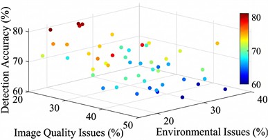
As an important part of power system operation and maintenance, power cable corrosion detection technology has experienced an evolution from manual inspection to intelligent analysis. Current research focuses on key facilities such as overhead lines, underground cables, and substation connections [12]. An analysis of current power patrol inspection technology is shown in Fig. 1.

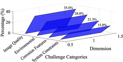
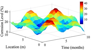
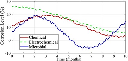
Fig. 1 summarizes the principal challenges in cable corrosion detection, highlighting the variability of corrosion levels across time and spatial locations, as well as the dependence of detection accuracy on image quality and environmental conditions.

Fig. 1Research status analysis of cable corrosion detection

a) 3D challenge distribution

b) 3D corrosion progression

c) Corrosion type progression

d) 3D accuracy vs challenges

Image quality factors account for 35 % of the challenges, encompassing issues such as insufficient resolution, motion-induced blur, and irregular illumination. Environmental interference constitutes 28 %, which involves complex backgrounds, significant occlusions, and adverse weather effects. Corrosion-specific characteristics represent 22 %, including morphological diversity, scale variance, and textural similarity. The remaining 15 % comprises system constraints such as real-time processing requirements and computational resource limitations. Collectively, these issues constitute the major impediments to the practical deployment of corrosion detection technologies [13].

3. Implementation of MSFEM-AAM for cable corrosion detection

The proposed YOLOv10-Transformer hybrid network adopts a dual-branch parallel structure. The backbone network, based on the CNN framework of YOLOv10, is responsible for extracting local features and spatial information. The Transformer branch serves as a complementary pathway, focusing on global dependency modeling. The outputs from both branches are fused through a feature alignment module to form complementary feature representations.

3.1. Hybrid network architecture design

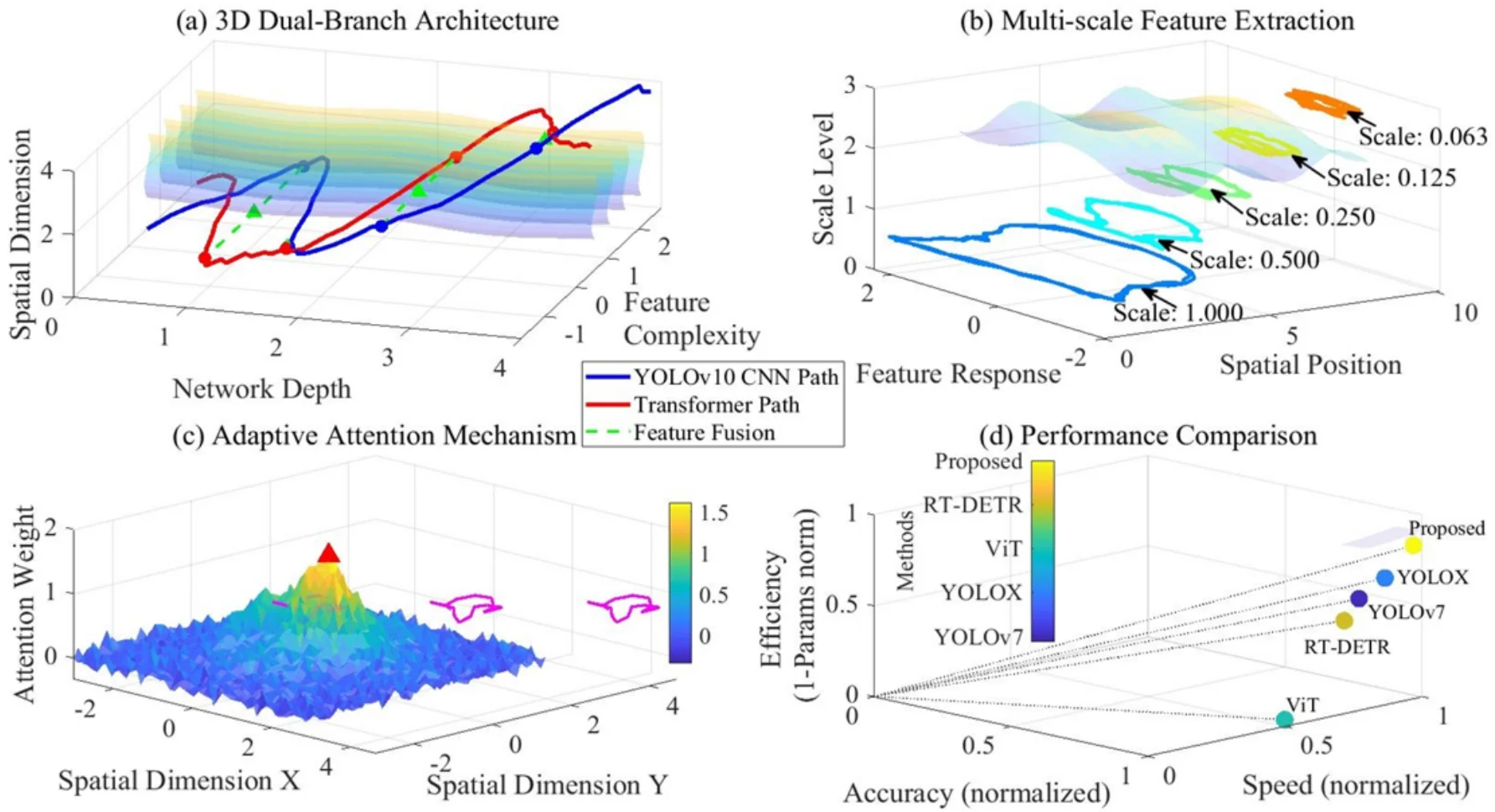
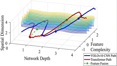
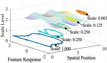
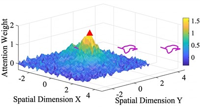
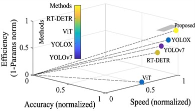
The hybrid network accepts three-channel cable images of size 640×640 as input. The YOLOv10 branch performs five downsampling operations to generate multi-scale feature maps, as illustrated in Fig. 2. Simultaneously, the Transformer branch partitions the input image into sequential patches of dimension 16×16, which are linearly projected into embedding vectors. Spatial information is preserved through positional encoding, while global context is learned via multi-layer encoders. The complete processing pipeline of the detection architecture is visualized in Fig. 2.

Fig. 2Improved YOLOv10-transformer hybrid network architecture

a) 3D dual-branch architecture

b) Multi-scale facture extraction

c) Adaptive attention mechanism

d) Performance comparison

Fig. 2 shows the parallel structure of the YOLOv10 CNN path and the Transformer path, including the spatial and channel attention weight distribution at feature fusion points and the performance comparison.

The network output contains information on the location, confidence, and classification of the corrosion area. The three detection scales respectively correspond to corrosion areas of different sizes to ensure that both large and small targets can be accurately identified. In the post-processing stage, weighted non-maximum suppression is used to effectively reduce overlapping frames while retaining the real target.

4. Evaluation model for cable corrosion state

The corrosion characterization framework establishes quantitative descriptors across three dimensions: textural, geometric, and spectral features. Textural attributes capture surface degradation patterns, geometric properties describe morphological alterations, and spectral signatures reflect compositional changes in materials. Task 1 – Corrosion Region Detection: The model locates corrosion areas in an image and classifies their severity. This is an object detection task. Its primary metric is mean average precision (mAP). Results are reported in Section 5.2.3. Task 2 – Corrosion Grade Classification: The model receives a cropped region (or an image containing a single corrosion area) and outputs a severity level: mild, moderate, or severe. This is a multi-class classification task. Its metrics are accuracy and macro F1-score. Results appear in Section 5.2.1. The two tasks share features extracted by the same backbone. Their outputs differ: Task 1 produces bounding boxes plus class labels; Task 2 produces only class probabilities.

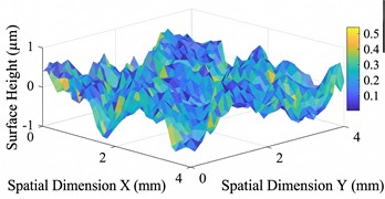
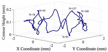
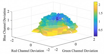
Collectively, these multi-dimensional features provide a comprehensive representation of corrosion states, as schematically illustrated in Fig. 3.

Fig. 3 presents the analysis of textural characteristics, demonstrating surface roughness and local binary pattern (LBP) features. Fractal dimension computation and corrosion profile complexity are evaluated, while spectral feature analysis reveals color deviation and variations in material composition. The distribution within the multidimensional feature space and the corresponding decision boundaries are also illustrated.

Fig. 3Corrosion feature quantification system: multi-dimensional analysis

a) 3D texture feature analysis

b) Geometric feature: fractal dimension = 1.168

c) Spectral feature: color deviation analysis

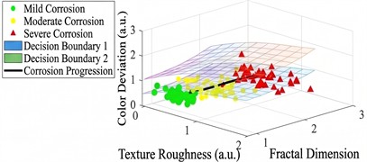
d) Multi-dimensional feature space

The preprocessing phase involves noise reduction and contrast enhancement, followed by postprocessing procedures that include feature fusion and dimensionality reduction:

where, $F_{texture}$ is the texture roughness, $N$ is the total number of pixels, and $\nabla I(x_i,y_i)$ is the gradient magnitude at position $(x_i,y_i)$.

This indicator is particularly sensitive to subtle texture changes caused by early corrosion:

where, $D_f$ is the fractal dimension, $N\left(ϵ\right)$ represents the contour length at scale $ϵ$, and $ϵ$ is the measurement scale.

This index effectively quantifies the roughness and self-similarity of the corrosion edge:

where, $C_{dev}$ is the color deviation, $M$ represents the number of sampling points, $H_j$ is the tone value of the $j$-th point, and $H_{ref}$ represents the reference tone value. The degree of color deviation measures the color difference between the corroded area and the normal area.

The model deployment considers the balance between computational efficiency and accuracy. In the feature extraction stage, the optimization algorithm is implemented, and fuzzy reasoning is accelerated using a lookup table method. These measures ensure that the system can meet real-time requirements.

5. Simulation experiment analysis

5.2. Analysis of simulation experiment

The experimental setup uses the parameters listed in Table 5 (lr = 0.001, Adam, MSE) to retrain the baseline models compared in Sections 5.2.1 to 5.2.3. This ensures consistency with the original implementation. However, the proposed MSFEM-AAM is trained with its own parameters (lr = 0.01, SGD, cosine annealing). Therefore, the goal is to compare the model architectures under the optimal settings of each model.

5.2.1. Corrosion grade classification accuracy comparison test

A comparative analysis against several contemporary state-of-the-art methods is performed to clearly delineate the quantitative performance positioning of our model in terms of classification capability. The comparative methods include Vision Transformer (ViT) [21], Convolutional Block Attention Module (CBAM) [22], and EfficientNet [23].

The calculation formula is as follows:

7

$Accuracy=\frac{N_{correct}}{N_{total}},$

where, $Accuracy$ is the classification accuracy, $N_{correct}$ is the number of samples correctly classified by the model, and $N_{total}$ is the total number of samples in the test set.

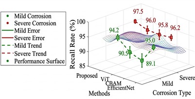
Macro F1-score is adopted to deal with possible category imbalance in the dataset. The experimental results are shown in Table 6 and Fig. 4.

Table 6Test results of corrosion class classification accuracy

Test items	The proposed model	ViT	CBAM	Efficient Net
Overall classification accuracy	96.8 %	95.1 %	94.3 %	95.5 %
Macro average F1 score	95.7 %	93.5 %	92.8 %	94.1 %
Mild corrosion recall	94.2 %	90.5 %	89.1 %	95.0 %
Heavy corrosion recall	97.5 %	96.0 %	95.8 %	96.2 %
Note: This table reports Task 2 (classification) performance. Detection results (mAP) are reported separately in Section 5.2.4

Fig. 4Comparative analysis of corrosion grade classification accuracy

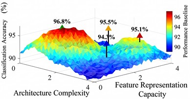
a) 3D performance landscape comparison

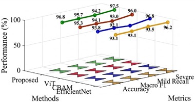
b) Multi-metric 3D performance comparison

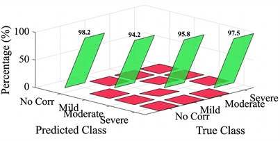
c) 3D confusion matrix- proposcd model

d) 3D recall performance with error bars

Fig. 4 illustrates the performance distribution of various methods within the space of architectural complexity and feature representation capability, including multi-metric performance profiles, confusion matrices, and recall performance.

The experimental results demonstrate that the confusion matrix of the proposed model exhibits the darkest hue along its main diagonal, indicating the highest consistency between its predictions and the ground-truth labels. The proposed model yields the optimal values in terms of both overall classification accuracy and macro F1-score. This suggests that the feature fusion mechanism incorporated in the model design effectively aggregates global and local information, thereby enhancing the confidence level of classification decisions. In practical applications, cable images are often subject to various degradation factors, such as noise, illumination variations, and partial occlusions. Tests are conducted to evaluate the robustness of the model under these non-ideal conditions.

5.2.2. Anti-interference robustness test

Cable images in practical applications are often disturbed by noise, illumination changes, and partial occlusion. Tests are designed to assess the robustness of the model under non-ideal conditions.

The test comparison methods include Denoising Convolutional Neural Network (DnCNN) [24], Adversarial Training [25], and ResNet [26].

The calculation formula is as follows:

8

$PerformanceDrop=\frac{P_{clean}-P_{noisy}}{P_{clean}}\times 100 \%,$

where, $PerformanceDrop$ represents the performance degradation rate, $P_{clean}$ is the macro F1-score of the model on the clean test set, and $P_{noisy}$ represents the macro F1-score of the model on the test set after adding interference.

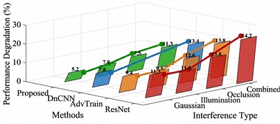
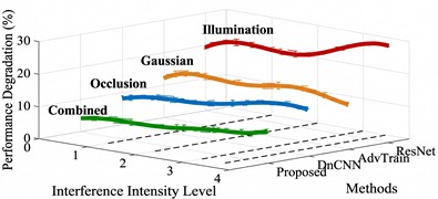
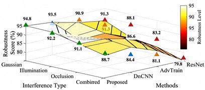
The experimental results are shown in Table 7 and Fig. 5.

Table 7Anti-interference robustness test results

Test items	The proposed model	DnCNN	Confrontation training	ResNet
Gaussian noise	5.2 %	7.8 %	9.1 %	12.5 %
Light mutation	6.5 %	–	8.7 %	11.9 %
Partial occlusion	8.9 %	–	13.4 %	16.8 %
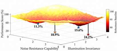
Integrated jamming	11.3 %	15.6 %	18.9 %	24.2 %

Fig. 5Comparative analysis of anti-interference robustness test

a) 3D robustness performance landscape

b) 3D Multi-interference degradation analysis

c) 3D degradation trajectory with uncertainty

d) 3D robustness comparison surface

Fig. 5 shows the distribution of robustness of different methods in the space of noise resistance and illumination invariance, including multi-interference degradation analysis, degradation trajectory and uncertainty, and a robustness comparison matrix.

The polygon corresponding to the model proposed in this study has the smallest area and is the closest to the coordinate origin, indicating that its performance degradation under various disturbances is the slightest. This demonstrates that the proposed model exhibits the minimum performance degradation rate and good robustness, making it more suitable for deployment in actual power scenarios with variable environmental conditions.

5.2.3. Computational complexity and inference efficiency test

The purpose of the test is to quantify the difference between the proposed model and the comparison methods in terms of computational complexity and actual inference time, and to assess the feasibility of their engineering applications. The test comparison methods include MobileNet [27], ShuffleNet [28], and Deep Separable Convolution [29].

The calculation formula is as follows:

9

$FLOPs=2\times H\times W\times C_{in}\times C_{out}\times K_h\times K_w,$

where, $FLOPs$ represents the number of floating-point operations of the convolutional layer; $H$ and $W$ are the height and width of the output feature map, respectively; $C_{in}$ is the number of input channels; $C_{out}$ is the number of output channels; and $K_h$ and $K_w$ are the height and width of the convolution kernel, respectively.

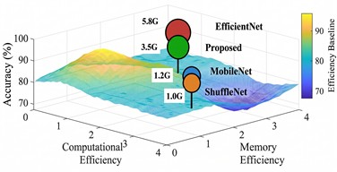
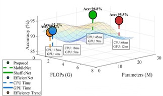
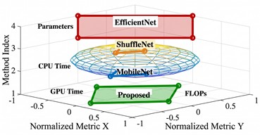
The experimental results are shown in Table 8 and Fig. 6.

Table 8Test results of computational complexity and inference efficiency

Test items	The proposed model	MobileNet	ShuffleNet	EfficientNet
Floating-point operations (FLOPs)	3.5G	1.2G	1.0G	5.8G
Number of parameters	15.3M	3.4M	2.8M	20.1M
CPU average inference time (ms)	45	18	15	68
GPU average inference time (ms)	9	5	4	12

Fig. 6Comprehensive analysis on computational complexity and inference efficiency

a) 3D computational efficiency landscape

b) 3D performance-resource trade-off

c) 3D computational complexity profiles

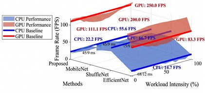
d) 3D real-time performance analysis

Fig. 6 displays the performance distribution in computational and memory efficiency space, including performance-resource trade-offs, computational complexity profiles, and real-time performance analysis.

The proposed model has higher computational complexity and parameter count than MobileNet and ShuffleNet, which are specifically designed for mobile platforms, yet it remains substantially lower than the bulky EfficientNet. Under GPU acceleration, it achieves an extremely short inference time of merely 9 milliseconds, fully meeting real-time processing requirements.

The inference latency of 9 ms per frame under GPU acceleration (NVIDIA RTX A6000) translates to a theoretical throughput of over 100 FPS, significantly surpassing the 25-30 FPS requirement typical for real-time video analysis. This performance margin provides a crucial buffer for practical deployment, accommodating potential overhead from preprocessing (e.g., video decoding, image stabilization) and postprocessing (e.g., alert generation, data logging) without compromising the system's real-time capabilities. When considering deployment on resource-constrained edge devices, however, the model's 15.3M parameters and 3.5G FLOPs present a challenge. Two primary strategies are envisaged for adaptation: first, the application of channel pruning to the convolutional layers, which could reduce the parameter count by an estimated 30-40 % with minimal accuracy trade-off; second, the quantization of weights from FP32 to INT8, a technique that demonstrably accelerates inference on edge TPUs. Such optimizations are essential for embedding the system onto inspection drones or portable handheld units.

The experimental results have demonstrated that the proposed model delivers comprehensive advantages in corrosion grade classification accuracy, robustness against disturbances, and computational efficiency. In terms of classification accuracy, the model outperforms contemporary state-of-the-art methods by approximately 1.3 % to 2.5 %, with particularly notable performance in identifying severe corrosion. During interference resistance tests, the model exhibits the lowest performance degradation rate under composite disturbances, reducing degradation by more than half compared to baseline models. Although computational efficiency is marginally lower than that of lightweight networks, the model still achieves real-time inference at 9 ms with GPU acceleration, effectively balancing accuracy and speed. These findings validate the efficacy of the model design.

6. Conclusions

In conclusion, we introduce MSFEM-AAM – a deep learning model for cable corrosion detection – which employs an innovative parallel architecture to enable simultaneous feature extraction and classification of corrosion images, thereby enhancing the operational efficiency of corrosion assessment in power cable inspection. Experiments conducted in a simulated environment indicate that MSFEM-AAM achieves a classification accuracy of 96.8 % with a noise immunity degradation rate of 11.3 %. Under GPU acceleration, the inference time is only 9 ms, which meets the real-time requirements of future power inspection tasks. These quantitative improvements indicate substantial breakthroughs in the model’s accuracy, robustness, and efficiency.

Beyond raw performance metrics, the system’s scalability for real-world deployment has been considered. The architecture’s modular design – where the YOLOv10 and Transformer branches function as semi-independent modules – facilitates future upgrades. For instance, the feature extractor could be swapped for a more efficient variant without necessitating a complete model redesign. Furthermore, the framework is inherently scalable to multi-sensor fusion. The current RGB-based detection could be extended by integrating a parallel processing stream for infrared thermal data using a similar dual-branch logic. This would allow the system to not only detect visible surface corrosion but also identify subsurface anomalies indicated by thermal differentials, thereby providing a more comprehensive assessment of cable health. Future work will focus on developing a lightweight, quantized version of this model specifically optimized for deployment on embedded platforms, followed by field trials to validate its robustness and long-term reliability in uncontrolled environmental conditions.

Currently, the model remains in the design phase and has not been deployed for practical validation. Therefore, future work will focus on model lightweighting for deployment on embedded devices, as well as extending the framework to multimodal data fusion by integrating infrared thermal imaging and ultrasonic testing, thereby enhancing the practical applicability of this innovative approach. Further research will investigate the model’s online learning capability in dynamic environments to achieve real-time corrosion monitoring and early warning. Additionally, we plan to explore the application of transfer learning in cross-domain corrosion detection, promoting the development of more versatile and intelligent assessment methodologies.