The approach for complexity analysis of multivariate time series

1. Introduction

Spatially extended complex dynamical systems, common in physics, biology and the social sciences such as economics, contains multiple interacting components and is nonlinear, non-stationary, and noisy, and one goal of data analysis is to detect, characterize, and possibly predict any events that can significantly affect the normal functioning of the system [1]. A lot of analysis techniques, originated from synchronization theory, nonlinear dynamics, information theory, statistical physics, and from the theory of stochastic processes, is available to estimate strength and direction of interactions from time series [2]. Among other techniques, the entropy measures are a powerful tool for the analysis of time series, as they allow describing the probability distributions of the possible state of a system, and therefore are capable to map changes of spatio-temporal patterns over time and detect early signs of transition from one to another regime. Various practical definitions and calculations of entropy exist [3-6], but most of them have been designed predominantly for the scalar case and are not suited for multivariate time series that are routinely measured in experimental and biological systems. Hence, suitable tools for the detection and quantitative description of the rich variety of modes that can be excited due to the interplay between spatial and temporal behavior are needed. Multivariate multiscale entropy (MMSE) has been recently suggested as a novel measure to characterize the complexity of multivariate time series [4]. The MMSE method involves multivariate sample entropy (MSampEn) and allows to account for both within- and cross-channel dependencies in multiple data channels. Furthermore, it operates over multiple temporal scales. The MMSE method is shown to provide an assessment of the underlying dynamical richness of multivariate observations and has more degrees of freedom in the analysis than standard MSE [4]. However, this MSampEn approach has limited application when the number of variables increases. Differently to the univariate sample entropy (SampEn) introduced by Richman and Moorman [5], which operates on delay vectors of a univariate time series, MSampEn calculates, for a fixed embedding dimension $m$, the average number of composite delay vector pairs that are within a fixed threshold $r$ and repeats the same calculation for the dimension ($m+1$) [4]. Because the composite delay vectors are high-dimensional (the dimension is equal to the product of the number of variables and the embedding dimension of the reconstructed phase space), the probability that at least two composite delay vectors will match with respect to tolerance $r$ quickly decreases as the number of variables increases. Among the other multivariate entropy approaches described is Multivariate Principal Subspace Entropy (MPSE) [6], introduced as a measure to estimate spatio-temporal complexity of functional magnetic resonance imaging (fMRI) time series. MPSE is based on the multivariate Gaussian density assumption of the fMRI data. Multivariate singular spectrum analysis (M-SSA) [7-10] provides insight into the dynamics of the underlying system by decomposing the delay-coordinate phase space of a given multivariate time series into a set of data-adaptive orthonormal components and is a powerful tool for spatiotemporal analysis of the vector-valued processes. M-SSA combines two useful approaches of statistical analysis: (1) it determines – with the help of principal component analysis – major directions in the system’s phase space that are populated by the multivariate time series; and (2) it extracts major spectral components by means of singular spectrum analysis (SSA). However, the Shannon entropy constructed from the M-SSA eigenvalue spectrum has weak distinguishing ability and does not provide information about the degree of complexity for both temporal and spatial components of multivariate time series.

In the present paper, it is shown that high-dimensional block Toeplitz covariance matrices (on which M-SSA operates) estimation via Kronecker product expansions makes it possible to define the complexity of multivariate time series by means of the spatial and temporal components and to obtain more information about the underlying process.

2. Description of the algorithm

Let $\mathbf{x}=\left\{x_d\left(n\right):d=1,\dots ,D,n=1,\dots ,N\right\}$ be a multivariate time series with $D$ components (variables) of length N. In practical implementation (neuroimagery with EEG, geosciences), this denotes samples of a space–time random process defined over a $D$-grid of space samples and an $N$-grid of time samples. It is assumed that each component has been centred and normalized. Each time series component of the multivariate system can be reconstructed in $M$-dimensional phase space by selecting the embedding dimension $M$ and time delay $\tau$. Each phase point in the phase space is thus defined by [11]:

where $n=1,2,\dots ,N-\left(M-1\right)\tau$, and ${\left(\bullet \right)}^T$ denotes the transpose of a real matrix. At $\tau =\text{1,}$ the reconstructed phase space matrix ${\mathbf{X}}_d$ with $M$ rows and $L=N-M+1$ columns (called a trajectory matrix) is defined by:

and encompasses $M$ delayed versions of each component. The total trajectory matrix of the multivariate system $\mathbf{X}$ will be a concatenation of the component trajectory matrices ${\mathbf{X}}_d$ computed for each component, that is, $\mathbf{X}={\left[{\mathbf{X}}_1,{\mathbf{X}}_2,\dots ,{\mathbf{X}}_D\right]}^T$, and has $DM$ rows of length $L=N-M+1$. The classical M-SSA algorithm [8, 9] then computes the covariance matrix $\mathbf{\Sigma }=1/L\bullet \mathbf{X}{\mathbf{X}}^T\in {\mathbb{R}}^{DM\times DM}$ of $\mathbf{X}$ and its eigendecomposition. The total trajectory matrix $\mathbf{X}$ can be rearranged such that the delayed versions of all $D$ components follow one another, that is, $\mathbf{X}={\left[{\mathbf{X}}_{D1},{\mathbf{X}}_{D2},\dots ,{\mathbf{X}}_{DM}\right]}^T$. In this case, and for $L\gg M$, the covariance matrix $\mathbf{\Sigma }\in {\mathbb{R}}^{MD\times MD}$ takes the block Toeplitz form:

with equal block submatrices ${\mathbf{\Sigma }}_Q\in {\mathbb{R}}^{D\times D}$ along each (top left to lower right) diagonal. The covariance matrix $\mathbf{\Sigma }$ combines all auto- as well as cross-covariances up to a time lag equal to $M-1$. The spatio-temporal covariance matrix $\mathbf{\Sigma }\in {\mathbb{R}}^{MD\times MD}$ can be represented as a Kronecker product (KP) [12-16]:

for some separation rank $r\text{,}$ some sequence of ${\mathbf{T}}_i\in {\mathbb{R}}^{M\times M}$ and ${\mathbf{S}}_i\in {\mathbb{R}}^{D\times D}\text{.}$ The KP parametrization assumes that an arbitrary spatio-temporal correlation can be modelled as a product of a spatial and a temporal factor. These two factors are independent of each other; hence, the spatial and temporal correlations are separated from each other in the KP model. The spatial covariance matrix captures the spatial correlations between the components of multivariate time series (in real-world application, signals registered at different sensors) and the temporal covariance matrix captures the temporal correlations as lag dependent. The meaning of Eq. (4) is that the temporal covariance matrix ${\mathbf{T}}_i$ is fixed in space and the spatial covariance matrix ${\mathbf{S}}_i$ does not vary over time. In other words, space and time are not correlated. In order to effective detect the structure of the spatio-temporal dependencies in high-dimensional multivariate systems, we use the full rank approximation model, i.e., define $r=M$. The solution to the nearest Kronecker product for a space-time covariance matrix (NKPST) problem is given by the singular value decomposition (SVD) of a permuted version of the space-time covariance matrix $\mathbf{\Sigma }\in {\mathbb{R}}^{MD\times MD}$ in the following:

1) The matrix $\mathbf{\Sigma }\in {\mathbb{R}}^{MD\times MD}$ is rearranged into another matrix $\mathbf{\Xi }\left(\mathbf{\Sigma }\right)\in {\mathbb{R}}^{M^2\times D^2}$ such that the sum of squares that arise in ${‖\mathbf{\Sigma }-\sum _{i=1}^r{\mathbf{T}}_i⨂{\mathbf{S}}_i‖}_F$ is exactly the same as the sum of squares that arise in ${‖\mathbf{\Xi }\left(\mathbf{\Sigma }\right)-\sum _{i=1}^r\mathrm{v}\mathrm{e}\mathrm{c}\left({\mathbf{T}}_i\right)⨂\mathrm{v}\mathrm{e}\mathrm{c}{\left({\mathbf{S}}_i\right)}^T‖}_F$, where $\mathrm{v}\mathrm{e}\mathrm{c}\left(\mathbf{W}\right)$ denotes the vectorized form of the square matrix $\mathbf{W}$ (concatenation of columns of $\mathbf{W}$ into a column vector). The $M^2$ rows of $\mathbf{\Xi }$ are defined as the transpose of the vectorized $D$×$D$ block submatrices of $\mathbf{\Sigma }$, where each block submatrix is ${\mathbf{\Sigma }}_Q\left(i,j\right)={\mathbf{\Sigma }}_{\left(i-1\right)D+1:iD,\left(j-1\right)D+1:D}$, $i$, $j=\text{1,}\text{…}\text{,}M$. That is, the permutation operator $\mathcal{R}:{\mathbb{R}}^{MD\times MD}\to {\mathbb{R}}^{M^2\times D^2}$ is defined by setting the $\left(\left(i-1\right)M+j\right)$th row of $\mathbf{\Xi }$ equal to $vec{\left({\mathbf{\Sigma }}_Q\left(i,j\right)\right)}^T$, $i$, $j=\text{1,}\text{…}\text{,}M$.

2) The SVD is performed on the matrix $\mathbf{\Xi }$:

and the matrices ${\mathbf{T}}_i$ and ${\mathbf{S}}_i$ are defined for the selected Kronecker product (full rank approximation) model by $\mathrm{v}\mathrm{e}\mathrm{c}\left({\mathbf{T}}_i\right)={\lambda }_i{\mathbf{u}}_i$ and $\mathrm{v}\mathrm{e}\mathrm{c}\left({\mathbf{S}}_i\right)={{\lambda }_i\mathbf{v}}_1$, where ${\mathbf{u}}_i$ and ${\mathbf{v}}_i$ are left and right singular vectors corresponding to the singular value ${\lambda }_i$ [13, 16]. This is converted back to a square ${\mathbf{T}}_i\in {\mathbb{R}}^{M\times M}$ and the ${\mathbf{S}}_i\in {\mathbb{R}}^{D\times D}$ matrix by applying the inverse permutation operator.

Finally, the SVD is performed on the estimated matrices ${\mathbf{T}}_i$ and ${\mathbf{S}}_i$, and the spatial and temporal components of the multivariate entropy (MVE) can be defined as the Shannon entropy of the corresponding normalized eigenvalue spectrum:

where ${\sigma }_{S,j}={\lambda }_{S,j}/\sum {\lambda }_{S,j}$ and ${\sigma }_{T,j}={\lambda }_{T,j}/\sum {\lambda }_T\text{,}$ are the summarized ${\lambda }_{S,j}=\sum _{i=1}^r{\lambda }_{S,j}^{\left(i\right)}\text{,}$${\lambda }_{T,j}=\sum _{i=1}^r{\lambda }_{T,j}^{\left(i\right)}$ and normalized eigenvalues of the decomposed matrices ${\mathbf{S}}_i$ and ${\mathbf{T}}_i$ respectively. The Shannon entropy quantifies the degree of uniformity in the distribution of the eigenvalues: it tends to unity at uniform distribution of the eigenvalues and tends to zero if the eigenvalue spectrum is concentrated into a single first largest eigenvalue. The entropy features $E_S$ and $E_T$ can be expressed in complex form $E_{\mathrm{\Sigma }}=E_{\mathrm{S}}+i{E}_T$, and the multivariate spatio-temporal entropy can be defined by modulus $\left|E_{\mathrm{\Sigma }}\right|$ and angle ${\phi }_E$ of this complex quantity. The angle ${\phi }_E$ reflects the difference between $E_S$ and $E_T$ and ranges from 0 (at $E_T=0$) to $\pi /2$ (at $E_S=0$).

3. Simulation results

To validate the ability of the proposed algorithm to reveal both within- and cross-component properties in multivariate data, we generated a multivariate time series with defined changes of the complexity. The overembedding ($M=$16) for all trials was chosen in order to capture the temporal properties of the time series. All data processing and analyses were performed using Matlab software (MathWorks, Natick, MA).

First, to illustrate the ability of the proposed algorithm to model cross-component properties in multivariate data, we considered a multivariate deterministic system – a chain of diffusively coupled Rössler oscillators [9, 17]:

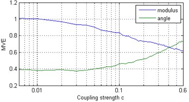
The position in the chain is given by the index $j=\text{1,…,}J$; ${\omega }_j={\omega }_1+0.02\left(j-1\right)$ are the associated natural frequencies, with ${\omega }_1=\text{1}$, and we assume that free boundary conditions $x_0\left(n\right)=x_1\left(n\right)$ and $x_{J+1}\left(n\right)=x_J\left(n\right)$ exist. The frequency mismatch ${\mathrm{\Delta }}_{jk}\omega$ between oscillators $j$ and $k$ is given by ${\mathrm{\Delta }}_{jk}\omega =0.02\left|j-k\right|$. The parameter $\alpha =\text{0.15}$, and $c\ge \text{0}$ is the coupling strength. We considered a chain of $J=\text{10}$ Rössler oscillators and generated a time series using the ODE45 integrator of Matlab. The solution was sampled at time intervals $t=$ 0.1, and the proposed algorithm was applied to $x$-components of length $N=$ 2048 of the Rössler systems. Fig. 1(a) shows the $\left|E_{\mathrm{\Sigma }}\right|$ and ${\phi }_E$ curves when the coupling strength $c$ is varied. As $c$ increases, the oscillators form synchronous clusters within which the observed frequency is the same [9]. With a further increase of $c$ the number of clusters decreases as clusters merge, and at sufficiently high c all oscillators are synchronized, i.e., all the mean frequencies coincide, although the amplitudes of the oscillators remain chaotic [17]. MVE is characterized by two components – modulus $\left|E_{\mathrm{\Sigma }}\right|$ and angle ${\phi }_E$ – that provide comprehensive information about the inherent structure of the multivariate data. The increasing value of ${\phi }_E$ indicates that $\left|E_{\Sigma }\right|$ decreases due to the growing strength of dependence between components of a multivariate time series.

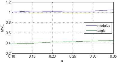
To illustrate the ability of the proposed algorithm to model within-component properties in multivariate data, we considered a chain of above-mentioned Rössler oscillators at $c=\text{0}$ and gradually increased the parameter $\alpha$ from 0.10 to 0.35. The larger $\alpha$, the more complex the resulting time series will be. The results are displayed in Fig. 1(b). In this case, the increased value of ${\phi }_E$ indicates that $\left|E_{\mathrm{\Sigma }}\right|$ slightly increases because of the degree of randomness of a time series.

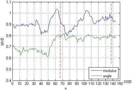
To demonstrate the performance of the proposed algorithm for quantifying changes in the dynamics underlying the experimental data set, we have applied the algorithm to multi-channel EEG recordings from epilepsy patients. It is well known that during epileptic seizures EEG time series display a marked change of the dynamics (mainly oscillations of comparatively large amplitude and well defined frequency). The EEG data with the clinically marked start and end of seizure are taken from the CHB-MIT Scalp EEG Database (http://www.physionet.org/physiobank/database/chbmit/). We analyzed 23 contacts of one-minute raw (unfiltered) scalp EEG recordings (from record, numbered chb01/chb01_04.edf) using the block Toeplitz covariance matrix, which was constructed over a moving window of length 3.9 s, corresponding to 1000 data points. This window was shifted with 90 % overlap over the whole EEG recording, and the time evolution of the $\left|E_{\mathrm{\Sigma }}\right|$ and ${\phi }_E$ was computed. As we can see in Fig. 2, both $\left|E_{\mathrm{\Sigma }}\right|$ and ${\phi }_E$ indicate sudden changes of the brain dynamics in preictal and ictal states. Furthermore, the angle ${\phi }_E$ of the multivariate entropy provides essential information about factors that cause this complicated dynamics. The considerable positive deviation of ${\phi }_E$ from its mean value denotes that $\left|E_{\mathrm{\Sigma }}\right|$ changes due to the growing strength of dependence between components of a multivariate time series, and also because of the degree of randomness of a time series.

Fig. 1Multivariate entropy (modulus EΣ and angle φE) for: a) a chain of coupled Rössler oscillators (x components) at various coupling strengths c; b) a chain of Rössler oscillators (x components) at c=0 and various values of parameter α

a)

b)

Fig. 2Multivariate entropy (modulus EΣ and angle φE) applied on epileptic EEG. The period between two vertical dashed lines is visually identified by the neurologists as the seizure period

4. Conclusion

A simulation involving a multivariate deterministic and stochastic time series shows that the approach based on a full rank Kronecker product expansion of the block-Toeplitz covariance matrix, calculated from the full augmented trajectory matrix, can reveal temporal dynamics and relationship between the signals; furthermore, it is a suitable tool for the assessment of the underlying dynamic complexity of multivariate observations. The proposed approach defined in terms of modulus and angle of the complex quantity constructed from the spatial and temporal components of the multivariate entropy reflects both the integrative properties of the systems and the ratio between the complexities in the spatial and temporal directions. The algorithm can be applied to the estimation of the complexity of multivariate time series with a large number (tens) of variates (e.g. EEG), when the application of the other approaches becomes problematic.