Abstract
As a novel time-frequency analysis method, adaptive local iterative filtering (ALIF) can decompose the time series into several stable components which contain the main fault information. In addition, the amplitude of singular value obtained by singular value decomposition (SVD) can reflect the energy distribution. Naturally, there are certain differences in the energy produced by different faults such as the broken tooth, wearing and normal. Thus, a novel method of mechanical fault classification method based on adaptive local iterative filtering and singular value decomposition is proposed in this paper. Firstly, ALIF method decomposed the original vibration signal into a number of stable components to establish an initial feature vector matrix. Then, the singular values energy corresponding to the feature matrix is employed as a criterion to identify various faults. Compared with the conventional EMD method by simulation experiments, ALIF method has obvious superiority in solving modal aliasing, which is more conducive to the advanced analysis. In this paper, the proposed method is employed to extract the fault information of rolling bearing fault signals from Case Western Reserve University Bearing Data Center. To further verify the effectiveness of the method, the case study is conducted at Drivetrain Diagnostics Simulator. To further illustrate the effectiveness of the method, the results obtained by this method are compared with EMD and EEMD. The results indicated the proposed method performs better in the classification of different mechanical faulty modes.
1. Introduction
Commonly, gears and rolling bearings are the most easily damaged parts in the mechanical equipment [1-6]. The working conditions of gears and rolling bearings are related to the security and stability of operation. Thus, it is important to detect and diagnose the running state of them. In most cases, gears and rolling bearings are running with high speed, heavy load or high temperature. Hence, the fault signal always has the characteristics of nonlinearity, nonstationary and non-Gaussian. Therefore, how to conduct the fault feature extraction from the non-stationary vibration signals is the critical process for fault diagnosis [7]. The traditional fault diagnosis method was analyzing the fault vibration signal in time-frequency domain to identify the states [8]. However, it is difficult to precisely diagnosis the working states only in time-frequency domain, due to the influence of non-linear factors such as load, friction, varying stiffness etc. Therefore, the improved signal processing methods based on data-driven should be considered.
The analysis of vibration signal is an important approach to monitor the running state of mechanical equipment, and it is more significant to accurately extract the fault feature frequency [9]. The collected vibration signals usually contain strong noise components, and the common method of beforehand noise reduction and reprocessing operation may lose some features and reduce the accuracy of signal reconstruction, resulting in false diagnosis conclusions. Due to the development of non-linear theory, many non-linear analysis methods have been proposed to deal with the problems of mechanical equipment fault diagnosis. For the processing of the non-linear and non-stationary signal, the current signal processing methods include Short-time Fourier Transform (STFT) [10, 11], Wavelet Transform (WT) [12-15] and Empirical Mode Decomposition (EMD) [16-18] etc. STFT is performed by selecting a window function, and assuming non-stationary signal to be stationary in the window. However, it requires that the analyzed signals in a short time interval. Essentially, it is still a smooth signal processing method, and the resolution is not high. WT is a multiscale signal analysis method based on STFT, which the width of the window function in the time axis translation process can be scalable. However, the selection of wavelet basis is hard to determine considering that the analyzed signals are presented with different characteristics. Moreover, after selecting the wavelet basis, the wavelet basis will remain unchanged during the processing, which lacks adaptability. Faced the above mentioned drawbacks, EMD has better performance. Huang et al. proposed a new signal analysis method to handle the non-linear and non-stationary problems, namely EMD. EMD can adaptively decompose a complex signal into a finite number of intrinsic mode functions (IMFs). Each IMF represents a set of characteristic scale signals. Furthermore, the energy which is extracted from each component can better reveal the inherent characteristics of fault information. However, this method can produce the problems of mode aliasing and uncertain order of the decomposition, which is harmful for feature extraction and different fault classification. To overcome the problem of mode mixing in EMD, Wu et al. [19, 20] proposed a noise assisted analysis method applied to the empirical mode decomposition namely ensemble empirical mode decomposition(EEMD), which can self-adaptively decompose a complicated signal into IMFs based on the local characteristic timescale of the signal. EEMD has two parameters to be set, which are the ensemble number m and the amplitude of the added white noise. However, this method produces more useless components. Cicone et al. [21, 22] presented a new adaptive time-frequency analysis method, namely adaptive local iterative filtering method(ALIF), which can be used to deal with nonlinear and non-stationary signals. ALIF is an adaptive decomposition method based on iterative filtering (IF). The difference between the two methods is that ALIF realizes adaptive decomposition of signals by choosing the length of the filters adaptively. ALIF can avoid the modal aliasing effectively and decompose the signals with same size and order.
According to matrix analysis theory, the singular value is the inherent characteristic of the matrix, which has a good stability [23, 24]. When there is a small change in matrix element, the singular value of the matrix changes a little [25, 26]. Moreover, the singular value of the matrix has the scale and rotation invariance. Accordingly, the singular value of the matrix satisfies the requirements of the stability, rotation and scale invariance in feature extraction of pattern recognition, which can effectively describe the characteristics of the initial feature vector matrix.
Since the influence of above non-linear factors and the complexity of the signal components, the faults of gear and rolling bearing parts are abnormal or different in the running process. The vibration signals obtained from the mechanical system will also change with the varied time, thus producing different energy signals. For gear and rolling bearing parts, different fault types always correspond to different degrees of vibration and complexity, which will lead to different energy values. Consequently, energy values can be used to classify different types of gear and rolling bearing faults. Thus, a novel fault classification method jointed adaptive local iterative filtering and singular value decomposition is proposed in this paper. Firstly, the vibration signal was decomposed into several components by ALIF, which was used to build an initial eigenvector matrix. Then, the singular value decomposition (SVD) was employed to decompose the initial feature vector to obtain the singular value, whose energy is selected as a criterion to identify various faults.
This paper was organized as follows: the basic principle and characteristics of the proposed fault classification method based on the singular value energy spectrum and adaptive local iterative filtering (ALIF) were introduced in the second chapter. In the third section, the numerical experiments were conducted, and then a simulation was operated to confirm the effectiveness of the proposed algorithm. In the fourth part, the validity of the proposed method was verified by processing the bearing data of the Case Western Reserve University [27] and the gear diagnosis simulator signals of application transmission system. The conclusions of the study and the necessary discussions were given in the fifth section.
2. The theory of the proposed method
2.1. The theory of adaptive local iterative filtering
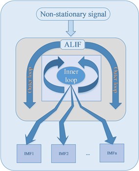
Adaptive local iterative filtering (ALIF) method is the improved version of iterative filtering [21]. The main difference between the two methods is that the former one can locally and adaptively calculate the length of filters and generates moving average line using the solution of Fokker Planck equation, which is so-called FP filter. Adaptive local iterative filtering method is as show in Fig. 1.
Given a signal and , we define , which represents the moving average function of the signal . In the above function, is a filter represented by step and the length is , in which . indicates that changes with .
Fig. 1The flowchart of adaptive local iterative filtering method
According to the definition of the moving average, we can also define an operator to capture the fluctuation of , in which the superscript reflects the number of IMF, thus the first IMF can be represented as .
There are two loops, an inner loop and an outer loop in the adaptive local iterative filtering algorithm. The inner loop is to capture a single IMF, and the outer loop is to generate all the IMFs of the signal. The iteration equation of the inner loop is shown as follows:
In order to establish the convergence theorem of ALIF algorithm, an equivalent formula is used to replace the previous calibration function. The calibration function can be represented as linearized or cubic form or any other function. With the help of , the above formula can be transformed into:
As a result, Eq. (1) can be written as the following form:
where () is a proper filter. We define a new operator:
Thus, the convergence theorem of the inner loop in ALIF algorithm is to make the continuous, in which and . Given that:
When approaches infinity, if accordingly, convergences to an IMF.
The convergence theorem of the outer loop in ALIF algorithm is that is continuous and differentiable, in which , and there is a finite number of extreme points in any small time interval of . Consequently, there are a maximum number of extreme points in . Given that , 1, 2,…, , are the extreme points of . is supposed strictly monotone in , and 1, 2,…, . Then, based on , function and can be defined as:
Assume that is a differentiable function with the above characteristics, it can be known from Eq. (2) that, if the scanning functions are separable, for example, , and for any :
If is in existence, the maximum number of extreme points in will be the number of extreme points in. For this convergence theorem, in the next step of the outer loop, the number of extreme points in is less than that of , meaning that is smoother than . If this feature maintains true in each of the outer loop, which means the number of extreme points of the remaining signal continues to decrease, as a result, for the signal, ALIF algorithm remains convergence.
2.2. The definition of singular value energy (SVE)
Singular value decomposition (SVD) is a typical orthogonal method. For a real matrix , there must be orthogonal matrix:
which will meet the following Eq. (7):
where and its transpose depends on the value of and , or , , 0 represents the zero matrix, , 0, and they are singular values of matrix .
Commonly, matrix can also be written as:
where , are respectively correspond to the column vector of and .
Thus, the singular value energy of the signal can be expressed as:
2.3. Feature extraction scheme based on adaptive local iterative filtering and singular value decomposition
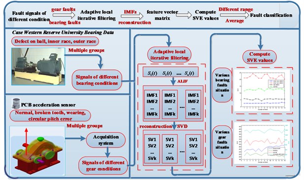
In this paper, a fault classification method based on ALIF for gear and rolling bearing is proposed. After experimental studies, it can be concluded that ALIF method has an obvious effect on denoising towards non-linear and non-stationary signal, etc. Thus, the ALIF method can be well applied to a variety of mechanical fault signals. As for gear and bearing parts, different fault types correspond to different fault degrees. From all above, ALIF method can be employed to decompose gear and bearing fault signals, and then apply SVE to conduct classification of different faults. The flowchart of the proposed method is illustrated in Fig. 2.
Fig. 2The flowchart of proposed method based on adaptive local iterative filtering and singular value decomposition
3. Numerical simulation analysis
Generally, the fault signal of rolling bearing and gear has a typical characteristic of non-linear and non-stationary. In order to illustrate the stability and effectiveness of the proposed method, a non-stationary signal with additive noise is used to simulate the actual situation. The expression of non-stationary signal is described as follows:
where the sampling frequency is set as 1000 Hz, the sampling length of each signal is determined as 5000. The random Gaussian noises are added with variance of 0.1 and average of 0. The time-domain diagram of , , are shown in Fig. 3.
Fig. 3Time-domain waveforms: a) signal x1, b) signal x2, c) signal f

a)

b)

c)
Fig. 4Decomposition results of f provided by EMD
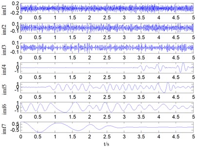
Fig. 5Decomposition results of f provided by EEMD
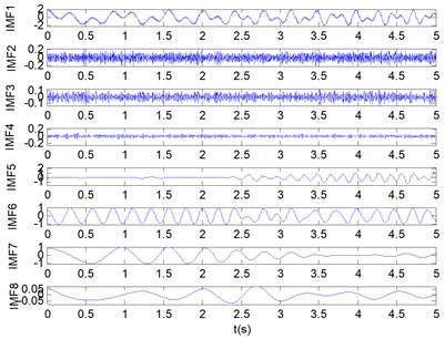
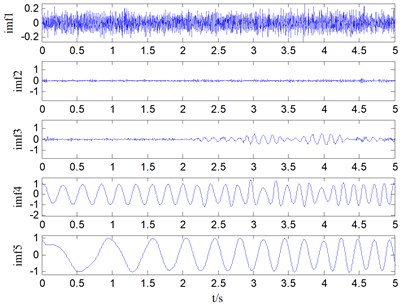
The EMD, EEMD and ALIF methods are employed to decompose the non-stationary signal . The results of the decomposition are shown in Fig. 4, Fig. 5 and Fig. 6 respectively. Fig. 4 shows the decomposition results contains nine IMFs and one residual component based on the EMD method. It can be seen that the result provided by EMD is not ideal compared with the original signal component. Similarly, the EEMD method decomposition results include twelve IMFs and one residual component, which is superior to EMD in terms of decomposition effect compared with EMD, as shown in Fig. 5 but the EEMD method produces more useless model components. The result derived from ALIF decomposition method is shown in Fig. 6. It is obvious that the proposed method has better effect on obtaining the original component, thus the decomposition results are preferable. From the above 3 diagrams we can see that the decomposition effect of ALIF method is more stable than EMD and EEMD.
Fig. 6Decomposition results of f provided by ALIF
4. Applications to gear and bearing fault classification
4.1. Application to processing of case western reserve university bearing data
Through numerical simulations, the proposed method based on adaptive local iterative filtering and singular value decomposition can be applied to the bearing signals. The fault bearing data from Case Western Reserve University Bearing Data Center Website [25] is used to verify the proposed method. The website provides a large collection of experimental bearing data that are related to faulty bearings, and among those the data for faulty bearings are acquired by using electric spark machining. In this paper, inner race, ball, and outer race fault data are both adopted. The sampling frequency in the experiment is 12000 Hz, and the rotational speed is 1730 rpm. Experimental fault bearing type is 6205-2RS JEM SKF, and its specific parameters are shown in Table 1.
Table 1Rolling element bearing parameters
Rolling element bearing parameters of 6205-2RS JEM SKF (diameter/mm) | |||||
Ball number | Contact angle | Ball diameter | Outside diameter | Inside diameter | Pitch diameter |
9 | 0 | 7.9 | 52 | 25 | 46.4 |
The test equipment of Case Western Reserve University includes two motors, a coupling (containing torque sensor and encoder), and other related devices. Accelerometer is placed on the testing site to collect acceleration signal that can be used for bearing fault analysis. The schematic diagram of a signal acquisition device and a picture are shown in Fig. 7.
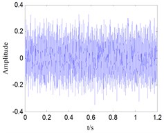
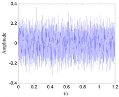
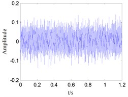
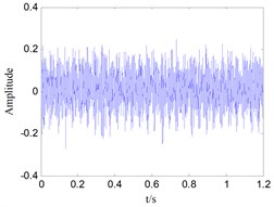
Generally, the collected signals such as rolling bearings of inner race, ball, and outer race contain many noise components. Then, the time-domain plots of one set of bearing signals are shown in Fig. 8. It is no doubt that the time-domain analysis of these groups of signals cannot clearly identify the difference between different kinds of faults.
Fig. 7The schematic diagram and a picture of the device: 1, 3 – Hp motor, 2 – torque transducer and encoder

Fig. 8Time-domain waveform of rolling bearing vibration signals with four states: a) inner race fault, b) outer race fault, c) roller fault, d) normal state
a)
b)
c)
d)
Empirical mode decomposition, ensemble empirical mode decomposition and adaptive local iterative filtering method are applied to decompose 15 groups of signals, and singular values of decomposed vibration signals are calculated, so as to conduct fault classification. The results are shown in Fig. 9, Fig. 10 and Fig. 11 respectively.
Fig. 9The singular value power of original signals decomposed by EMD
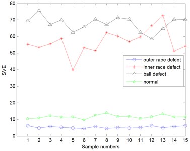
Fig. 10The singular value power of original signals decomposed by EEMD
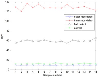
Based on the previous several mode decomposition algorithms, the decomposed components will constitute an initial feature matrix to express the signal energy and then the singular values of initial feature matrix are calculated. Through the mode decomposition and feature reconstruction of the original signal, it can be shown from the Fig. 9 that the SVE value of the working condition is not different from the other working state in the result obtained by the EMD. Inside, the inner race and the rolling element already have some aliasing. Similarly, the EEMD method was used to decompose the vibration signals and the SVE values were shown in Fig. 10. It can discriminate the inner race fault and rolling element defect, however, the SVE values of the outer race fault and the normal is not clearly. However, the bearing vibration signals are decomposed by the ALIF, the SVE of bearing signals of four kinds of working conditions are distinguished very clearly from the Fig. 11.
Fig. 11The singular value power of original signals decomposed by ALIF
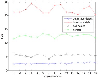
In order to explain the classification effect of faults more accurately, the fault accuracy is used to evaluate the classification results of several methods. From the result graph of EMD decomposition, we can see that 2 groups of rolling element and outer race have been mixed, and the total sample number is 15 groups, so the classification accuracy is 86.67 %. From the decomposition effect of EEMD, we can see that the boundary between the inner ring and the rolling body is obvious, as shown in Fig. 10, and the boundary between the normal and outer race is very vague. One of the groups has been coincident, so the classification accuracy is 93.33 %. However, the results of ALIF decomposition can be divided into several kinds of faults, and the boundary between them is obvious, and the classification accuracy is close to 100 %.
Table 2SVE values under different conditions
Working Condition | Maximum SVE | Minimum SVE | Average SVE |
Normal | 13.42 | 11.56 | 12.56 |
Outer race fault | 5.94 | 4.25 | 5.51 |
Inner fault | 24.28 | 20.29 | 21.98 |
Rolling element | 3.15 | 2.42 | 2.62 |
As shown in Table 2, the rolling element energy value is the smallest, which the energy value varies from 2.42 to 3.15 and the average value is 2.62. Furthermore, the energy value of fault vibration signal about normal bearing varies from 11.56 to 13.42 and the average value is 12.56. The energy value with the inner fault vibration signal is changed from 20.29 to 24.28 and the average value is calculated as 21.98. Moreover, the energy value about outer race fault vibration signal is from 4.25 to 5.94 and the average value is calculated as 5.51. It is illustrated that different fault types correspond to different energy average values and ranges, which can be used to classify different types of mechanical fault modes. Therefore, it can be concluded that several groups of bearing signals under different types of operating conditions can be classified by the proposed method.
4.2. Application to drivetrain diagnostics simulator
Through the simulation analysis, the proposed fault classification method based on adaptive local iterative filtering (ALIF) and singular value decomposition (SVD) is applied to the experimental gear signals. Owing to the unqualified manufacture or improper manipulation, different kinds of gear faults would occur during the operation process. In the studies of this paper, the collected different fault signals of Drivetrain Diagnostics Simulator are adopted to verify the effectiveness of the proposed method. The experimental apparatus has a single stage of gear transmission. The small gear is installed on the input shaft with tooth 20, and the big gear is installed on the output shaft with tooth 37. The module of gears is determined as 3. The load is generated by the magnetic powder brake, and the acceleration sensor is installed on bearing pedestal of the input shaft in a vertical direction. Under different working conditions, several group signals as normal gear, broken tooth, wearing and circular pitch error gear vibration signals, were collected. There is a significant crack in the root of the broken tooth, the depth account tooth thickness of 2/5. The wearing tooth is produced by a distinct wear on the gear surface. The specific parameters of test conditions are described as follows: the speed of high-speed shaft is 363 r/min, and the load is 0 when the apparatus is idle, the sampling frequency and time are set as 2000 Hz and 3 s respectively. Thus, each set of data has 6000 sampling points. The experimental apparatus and its schematic diagram are shown in Fig. 12. The apparatus contains a variable speed drive, a single stage gear transmission, and a magnetic powder brake.
Fig. 12The schematic diagram and a picture of the experimental apparatus: 1 – magnetic powder brake, 2 – single stage gear transmission, 3 – variable speed drive
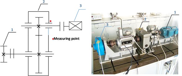
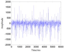
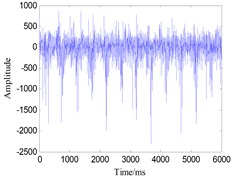
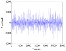
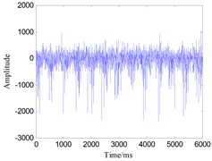
Fig. 13Time-domain waveform of gear vibration signals with four states: a) broken tooth, b) wearing, c) circular pitch error, d) normal state
a)
b)
c)
d)
Since this apparatus is small and has a high rigidity, the collected signals such as normal gear, broken tooth, wearing and circular pitch error signals are all affected by vibration of the foundation bolts. The time-domain plots of one set of gear signals are shown in Fig. 13. The spectral analysis of these groups of signals cannot demonstrate obvious differences between different kinds of faults.
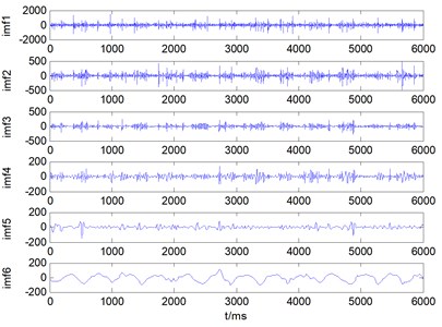
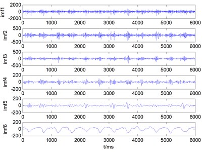
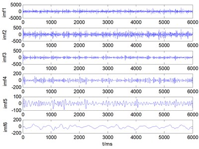
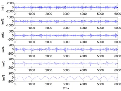
The 15 groups of signals correspond to each faulty mode are decomposed by the above methods. A set of mode decomposition result provided by ALIF is plotted in the following Fig. 14. Then, the energy value of the decomposed signal is calculated, so as to conduct the different fault classification. The results of classification are shown in Fig. 17. In order to verify the effectiveness of the proposed method, the EMD and EEMD methods are also used to decompose the above signals, and the results are shown in Fig. 15 and Fig. 16 respectively.
By decomposing the original fault signal into several modes by the above methods, the obtained mode components are formed into an initial characteristic matrix. Then the singular value of the initial characteristic matrix is used to calculate the signal energy. As shown in Fig. 15, the SVE value of the working condition is not different from the other working state in the result obtained by the EMD. Inside, the Pitch error and the normal already have some aliasing.
Fig. 14A set of mode decomposition result provided by ALIF: a) broken tooth, b) wearing, c) circular pitch error, d) normal state
a)
b)
c)
d)
The result of EEMD is better than that of EMD. We can see from the Fig. 16 that it can distinguish the pitch error, the normal and the broken teeth, but there are still 2 sets of aliasing between the broken teeth and the wear. However, the gear vibration signals are decomposed by the ALIF, and the SVE of the gear signal under four working conditions with the energy division has obvious diversity from the Fig. 17.
Just like the former, in order to explain the classification results more accurately, the classification accuracy of EMD and EEMD methods is 60 % and 86.67 % respectively. It is worth mentioning that the classification accuracy of ALIF decomposition is close to 100 %.
Fig. 15The singular value power of original signals decomposed by EMD
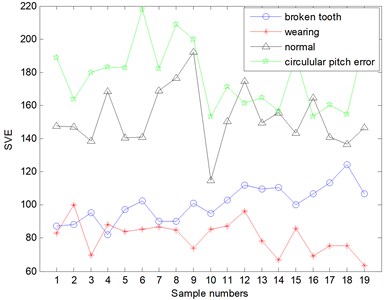
Fig. 16The singular value power of original signals decomposed by EEMD
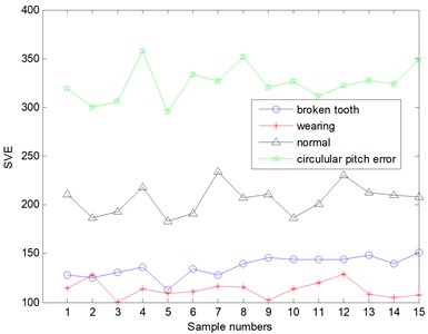
Fig. 17The singular value power of original signals decomposed by ALIF
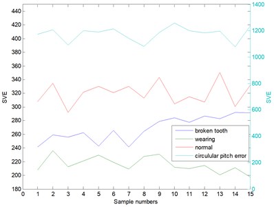
As shown in Table 3, the SVE of vibration signals of pitch error are the largest, ranging from 1079.1 to 1257.1, and their mean value is 1176.3. The SVE of normal gear varies from 291.77 to 350.57, and the average value is 320.24. The SVE of broken gear is changed from 241.44 to 292.26, and their mean value is 268.40. Moreover, the SVE of wearing gear are smallest, ranging from 235.91 to 197.59, and their average value is 216.02. The different singular value energy with each fault types can be performed as criterion of fault classification. Therefore, the proposed method can be used to classify different faulty modes under different working conditions.
Table 3SVE values under different conditions
Working Condition | Maximum SVE | Minimum SVE | Average SVE |
Wearing | 235.91 | 197.59 | 216.02 |
Broken tooth | 292.26 | 241.44 | 268.40 |
Normal | 350.57 | 291.77 | 320.24 |
Pitch error | 1257.1 | 1079.1 | 1176.3 |
5. Conclusions
The research work in this paper elaborates on the theoretical effectiveness of the proposed method based on the adaptive local iterative filtering (ALIF) and singular value decomposition (SVD). The simulation results demonstrated that ALIF could avoid the mode mixing and not produce more useless components. By applying the proposed method to the analysis of fault bearing signal from the West Reserve University public data-set and the Drivetrain Diagnostics Simulator, the characteristic of the gears and rolling bearings under different fault types could be clearly separated. The significance of the proposed method in the field of fault classification can be proved. Therefore, it can be concluded that several groups of gear and bearing signals under different types of working conditions can be classified by the proposed method, which can identify and diagnose the gear and bearing fault. In order to further illustrate the effectiveness of the method, the results of classification are compared with the results of EMD and EEMD decomposition respectively. Experimental results show that the proposed method is better than EMD and EEMD. From all above, it clearly indicates that the proposed method is a successful exploration.
References
-
Lv Y., He B., Yi C., et al. A novel scheme on multi-channel mechanical fault signal diagnosis based on augmented quaternion singular spectrum analysis. Journal of Vibroengineering, Vol. 19, Issue 2, 2017, p. 955-966.
-
Yi C., Lv Y., Dang Z., et al. Quaternion singular spectrum analysis using convex optimization and its application to fault diagnosis of rolling bearing. Measurement, Vol. 103, 2017, p. 321-332.
-
Zimroz R., Bartelmus W., Barszcz T., et al. Diagnostics of bearings in presence of strong operating conditions non-stationarity a procedure of load-dependent features processing with application to wind turbine bearings. Mechanical Systems and Signal Processing, Vol. 46, Issue 1, 2014, p. 16-27.
-
Tang H., Chen J., Dong G. Dynamic linear models-based time series decomposition and its application on bearing fault diagnosis. Journal of Vibration and Control, Vol. 21, Issue 5, 2015, p. 975-988.
-
Yi C., Lv Y., Ge M., et al. Tensor singular spectrum decomposition algorithm based on permutation entropy for rolling bearing fault diagnosis. Entropy, Vol. 19, Issue 4, 2017, p. 139.
-
Michele C. Application of Dang Van criterion to rolling contact fatigue in wind turbine roller bearings under elastohydrodynamic lubrication conditions. Proceedings of IMechE, Part C: J Mechanical Engineering Science, Vol. 228, 2014, p. 2079-2089.
-
Feng X. L., Wang G. F., Qin X. D., et al. The comparison of acoustic emission with vibration for fault diagnosis of the bearing. Applied Mechanics and Materials, Vol. 141, 2012, p. 539-543.
-
Feng Z., Liang M., Chu F. Recent advances in time-frequency analysis methods for machinery fault diagnosis: a review with application examples. Mechanical Systems and Signal Processing, Vol. 38, Issue 1, 2013, p. 165-205.
-
Lv Y., Yuan R., Song G. Multivariate empirical mode decomposition and its application to fault diagnosis of rolling bearing. Mechanical Systems and Signal Processing, Vol. 81, 2016, p. 219-234.
-
Sharma G. K., Kumar A., Rao C. B., et al. Short time Fourier transform analysis for understanding frequency dependent attenuation in austenitic stainless steel. NDT&E International, Vol. 53, 2013, p. 1-7.
-
Balazs P., Bayer D., Jaillet F., et al. The pole behavior of the phase derivative of the short-time Fourier transform. Applied and Computational Harmonic Analysis, Vol. 40, Issue 3, 2016, p. 610-621.
-
Lau E. C. C., Ngan H. W. Detection of motor bearing outer raceway defect by wavelet packet transformed motor current signature analysis. IEEE Transactions on Instrumentation and measurement, Vol. 59, Issue 10, 2010, p. 2683-2690.
-
Yan R., Gao R. X., Chen X. Wavelets for fault diagnosis of rotary machines: A review with applications. Signal Processing, Vol. 96, 2014, p. 1-15.
-
He W., Yi C., Li Y., Xiao H. Research on mechanical fault diagnosis scheme based on improved wavelet total variation denoising. Shock and Vibration, 2016, p. 3151802.
-
Kankar P. K., Sharma S. C., Harsha S. P. Rolling element bearing fault diagnosis using wavelet transform. Neurocomputing, Vol. 74, Issue 10, 2011, p. 1638-1645.
-
Huang N. E., Steven Z., Long S. R., et al. The empirical mode decomposition and the Hilbert spectrum for nonlinear and non-stationary time series analysis. Proceedings of the Royal Society of London-A, Vol. 454, Issue 1971, 1998, p. 903-995.
-
Gilles J. Empirical wavelet transform. IEEE Transactions on Signal Processing, Vol. 61, Issue 16, 2013, p. 3999-4010.
-
Ricci R., Pennacchi P. Diagnostics of gear faults based on EMD and automatic selection of intrinsic mode functions. Mechanical Systems and Signal Processing, Vol. 25, Issue 3, 2011, p. 821-838.
-
Wu Z., Huang N. E. A study of the characteristics of white noise using the empirical mode decomposition method. Proceedings of the Royal Society of London A: Mathematical, Physical and Engineering Sciences, The Royal Society, Vol. 460, Issue 2046, 2004, p. 1597-1611.
-
Wu Z., Huang N. E. Ensemble empirical mode decomposition: a noise-assisted data analysis method. Advances in Adaptive Data Analysis, Vol. 1, Issue 1, 2009, p. 1-41.
-
Cicone A., Liu J., Zhou H. Adaptive local iterative filtering for signal decomposition and instantaneous frequency analysis. Applied and Computational Harmonic Analysis, Vol. 41, Issue 2, 2016, p. 384-411.
-
Cicone A., Liu J., Zhou H. Adaptive local iterative filtering for signal decomposition. Applied and Computational Harmonic Analysis, Vol. 41, Issue 2, 2016, p. 384-411.
-
Rufai A. M., Anbarjafari G., Demirel H. Lossy image compression using singular value decomposition and wavelet difference reduction. Digital Signal Processing, Vol. 24, 2014, p. 117-123.
-
Sun C., Raghunathan S., Husbands P. J. R., et al. Singular Value Decomposition of Complex Matrix. U.S. Patent 9, 2016.
-
Yi C., Lv Y., Xiao H., et al. Laser induced breakdown spectroscopy for quantitative analysis based on low-rank matrix approximations. Journal of Analytical Atomic Spectrometry, Vol. 32, 2017, p. 2164-2172.
-
Zhang W., Zhu J., Pu Y., et al. Application of singular value energy difference spectrum in axis trace refinement. Sensors and Transducers, Vol. 167, Issue 3, 2014, p. 55-60.
-
Loparo K. A. Bearings Vibration Data Set. Case Western Reserve University, http://csegroups.case.edu/bearingdatacenter/home.
About this article
This work was supported by the National Natural Science Foundation of China under Grants No. 51475339, the Natural Science Foundation of Hubei province under Grant No. 2016CFA042, the Applied Basic Research Programs of Wuhan science and technology bureau under Grants No. 2017010201010115, and the Engineering Research Center for Metallurgical Automation and Measurement Technology of Ministry of Education (Wuhan University of Science and Technology) Grants No. MARC201701. The authors also appreciate the free download of the original bearing failure data and one photo picture provided by Case Western Reserve University Bearing Data Center Website.
Yong Lv and Yi Zhang conceived and designed the experiments. Yong Lv and Cancan Yi performed the experiments. Yong Lv and Han Xiao analyzed the data. Cancan Yi and Zhang Dang contributed reagents/materials/analysis tools. Cancan Yi and Yi Zhang wrote the paper.
