Abstract
Vibration signals of rolling element bearings during operation are always very complex, random strongly and broadband. Adaptive Local Iterative Filtering Decomposition (ALIFD) can overcome the smoothness and adaptive flaws of Iterative Filtering Decomposition (IFD), but it is so susceptible to random noise that it’s less effective. Here, spatial correlation was proposed. Firstly, the signal was denoised by spatial correlation and decomposed into several modes by ALIFD. Finally, the envelope demodulation was analyzed to extract fault feature. The simulating signal analysis and bearing fault simulator show that this method can be available for separating different frequencies of bearing fault vibration signals.
Highlights
- Spatial correlation can keep signal details at the same time, effectively reduce noise, and improve the SNR
- ALIFD is an adaptive time-frequency method analyzed the nonlinear and non-stationary signals, and remains locality, adaptability and stability
- The simulating analysis and experiments show that this method based on Spatial Correlation and ALIFD can be available for bearing fault diagnosis
1. Introduction
Vibration signals of rolling element bearings during operation are always very complex and random broadband [1]. What’s more, different reasons result in different bearing system incentives. For example, the incentive, which is caused by the surface damage (fatigue pitting or peeling) of the bearing components, is a shock. So the vibration signal is the carrier of bearing fault, and the fault location can theoretically be diagnosed through the analysis of the bearing vibration signal. When there is a local fault in rolling bearing, there are the nonlinear and non-stationary characteristics and periodic pulse in vibration signals of bearings. The traditional signal analysis technology is difficult to achieve remarkable results. For instance, Fourier transform is more suitable for periodic or stationary and linear system [2]. Wavelet transform needs to predefine basis function, and cannot meet the adaptive requirements [3]. In practical application, this pulse has a lower energy proportion, and is vulnerable to be interfered by background noise. Especially in the early bearing failure, fault characteristics are faint, making it not easy to identify and extract the periodic pulse in the background noise. Single fault diagnosis methods fail to show good effect [4-7]. Therefore, what kind of vibration monitoring and signal processing technology used to effectively extract the bearing fault characteristic information becomes the key of the bearing fault diagnosis [8].
In order to extract the features of the bearing fault vibration signal, the time-frequency analysis based on signal decomposition is widely used in recent years [9]. Empirical Mode Decomposition (EMD) works as a nonlinear and non-stationary signal analysis which doesn't need to be predetermined basis-functions and has the completeness, orthogonality and adaptability, so it is widely used in fault diagnosis of rolling bearing [10]. But this method also has limitations, such as end effects, incomplete envelope and mode mixing. Luan Lin et al. built a low-pass Filtering function and proposed the IFD [11]. However, the compact support low pass filters used in the existing IFD are not smooth enough. Antonio Cicone et al. designed smooth filters with compact support from solutions of Fokker–Planck equations (FP filters) in order to realize a local, adaptive and stable iterative filtering, and proposed the ALIFD [12].
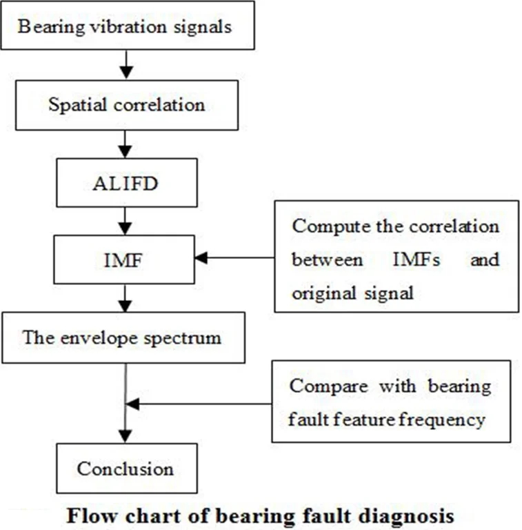
The actual vibration signal in addition to reflecting the bearing working condition, also contains a large number of background noise, which produced by other moving parts in machinery and structure. Owing to the strong background noise, the early fault feature is often buried and is difficult to extract. Spatial correlation denoising method based on correlation information of wavelet coefficient in a variety of scale and product with the coefficient of the neighboring scales, can suppress noise and sharpen edges effect [13]. Therefore, this paper combined the advantages of spatial correlation and ALIFD, and then proposed rolling bearing fault feature extraction based on spatial correlation and ALIFD. Firstly, the signal was denoised by spatial correlation and decomposed into several Intrinsic Mode Functions (IMFs) by ALIFD. Finally, the envelope demodulation was analyzed to extract different frequencies of bearing fault vibration signals and diagnose bearing fault location.
2. Spatial correlation
2.1. The principle of spatial correlation
Given a simple signal:
where is the original signal and is the noise [14].
(1) The signal is decomposed by wavelet transform to get wavelet coefficients with indexing position and indexing scale, where is the corresponding wavelet coefficients of original signal and is the corresponding wavelet coefficients of noise . By normalizing and comparing their absolute values with . If , ; If , .
(2) Repeat steps (1) until is nearly equal to a threshold associated with noise level, and , where is the norm of mother wavelet and is the noise variance in indexing scale.
(3) is the target decomposition coefficient and is reconstructed to get the denoised signal by spatial correlation.
The wavelet coefficients of fault signals after wavelet transform have strong correlation between the various scales, especially stronger on the edge of the signal correlation, which the corresponding correlation of noise is relatively weak. Spatial correlation method can achieve the noise reduction while the fault signal and the noise have different characteristics of spatial correlation on the scale wavelet coefficients.
Fig. 1Time-domain waveform of the simulation signal
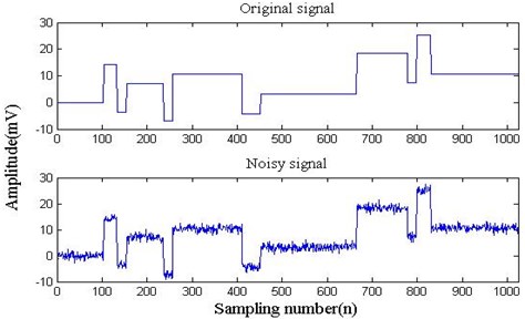
2.2. Comparison analysis of spatial correlation and wavelet shrinkage denoising
The noise signal, whose signal-to-noise ratio (SNR) is 7, is constructed by noise function of MATLAB. The time domain waveform of original signal and added noise signal are shown in Fig. 1. The signal is decomposited into 5 level to get the waveform of high frequency coefficients by wavelet transform and spatial correlation respectively, which is shown in Fig. 2.
Fig. 2Waveform of high frequency coefficients and high frequency coefficients after spatial correlation denoising
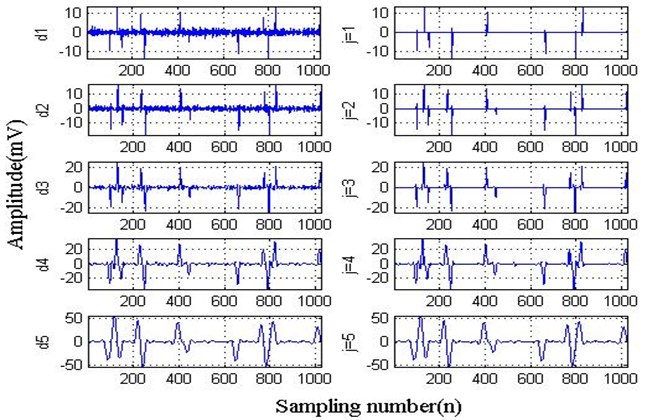
Fig. 3 is the denoised signal after reconstruction, and the SNR of spatial correlation filtering signal is 47 and the SNR of threshold filtering signal is 17. So SNR by spatial correlation is improved obviously and noise is effectively restrained in Table 1; what’s more, this method has an obvious advantage over threshold filtering, improves SNR greatly, and has high level of the closeness and smoothness.
Fig. 3Two methods of signal denoising
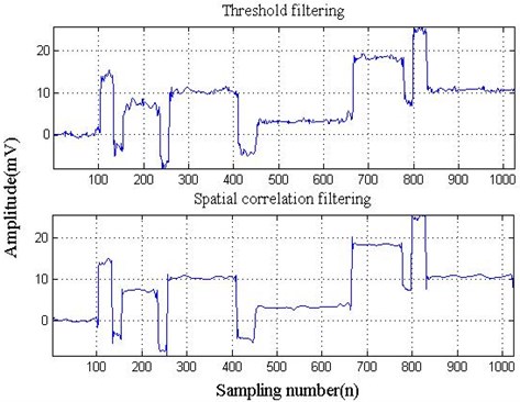
Table 1Signals’ SNR
Signal | SNR |
The simulation signal | 7 |
Threshold filtering signal | 17 |
Spatial correlation filtering signal | 47 |
3. Adaptive local iterative filtering decomposition (ALIFD)
3.1. The principle of ALIFD
Given two derivable functions and , then [12]:
1) 0, 0 and ;
2) .
Let us consider the Fokker-Planck equation:
where , are steady-state coefficient and , .
The of Ep. (1) generates diffusion effect and pulls out the solution from the center towards endpoint, while the term transports it from endpoint towards the center of the interval. When the two forces are balanced:
satisfying 0 for , and 0 for . That means the solution is concentrated in the interval [] and is a local filter.
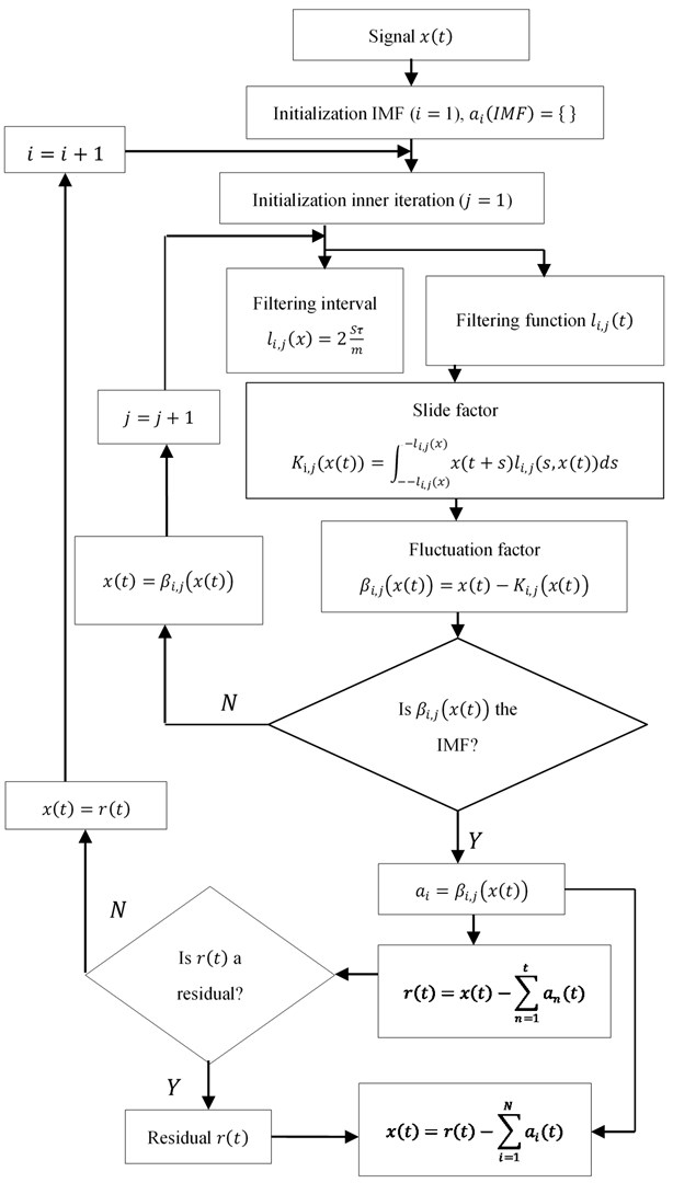
The ALIF method has two iterations: the inner iteration, to capture each single IMF, and the outer iteration to produce all the IMFs. The specific process can be shown as follows in Fig. 4.
3.2. The inner iteration
Firstly, the sliding operator computed by Ep. (4) is the convolution of signal and filtering function :
where is the total sample points of signal , is the number of its extreme points, is a parameter usually fixed around 1.6.
The sliding operator computed by Ep. (4) is extracted from signal to obtain fluctuations operator :
while the fluctuation factor can meet IMF’s requirements, is the IMF. But the initial does not meet the conditions, IMFs corresponding to frequency oscillations were carefully chosen by a more restrictive stopping criterion.
3.2.1. The outer iteration
To produce the -th IMF, we apply the previous process to the residual signal , and the algorithm stops when r becomes a trend signal, meaning it has at most one local extreme:
On account of space limitations, no specific deduction is given. Please refer to reference [15] for details.
Fig. 4Flow chart of ALIFD
3.3. Comparison analysis of simulation signals
Given the simulation signals:
where sampling number is 5000, and [0, 2].
Fig. 5 is the waveform of simulation signal , and , which are also the ideal IMFs of the signal decomposition, but the fact is not necessarily consistent with them.
Fig. 5The waveform of simulated signal
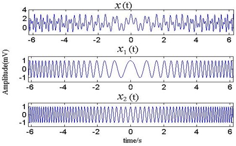
Fig. 6The waveform of EMD
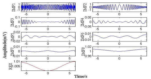
Fig. 7The waveform of IFD
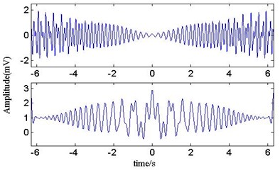
Fig. 8The waveform of ALIFD
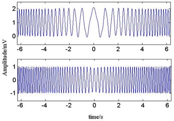
Fig. 6 is the result of EMD. It shows that the IMF1, IMF2 decomposed by EMD are simply similar to and in the middle. Because the instantaneous frequency between the two signals has overlapping portion, this makes a difference on both ends of the signal, and the original signal waveform component is not decomposed completely. Meanwhile, some mistakes appear in the result of the decomposition, which complicates the signal analysis. Fig. 7 is the result of IFD. It is evident that the IMF1, IMF2 decomposed by IFD have great difference with and . Because of the overlapping portion of instantaneous frequency between the two signals, IFD can change adaptively filter length according to the signal features. Fig. 8 is the result of ALIFD. Because ALIFD sets out from point to point changing adaptively the filter length to realize the signal decomposition, and does not need to know any information about signal in advance, but also can filter the small amplitude oscillation of the signal and the derivation process. So the IMFs decomposed by ALIFD coincide with and .
4. Numerical simulation
To verify the effectiveness of the proposed method, a mixed signal is studied:
where 3000 Hz is carrier frequency, 5 is displacement constant, 0.1 is damping coefficient, 0.01 s is the period of impact, 20 kHz is the sampling frequency, 4096 is the sampling number, is the sampling time, and is white noise with variance of 2.
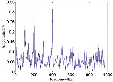
As shown in Fig. 9, it is the waveform of simulation signal. Due to the influence of noise, it is very hard to identify the bearing fault feature. To test the validity of the method uniting the spatial correlation with ALIFD, the signal and denoised signal by the spatial correlation are decomposed by ALIFD respectively. The denoised signal by the spatial correlation is processed by ALIFD, and then analyzed the envelope spectrum of the first IMF. From the Fig. 10, the impact frequency (100 Hz) and its harmonic (200 Hz, 300 Hz, 400 Hz, 500 Hz, etc.) can be shown. However, the simulation signals are decomposed by ALIFD directly, and the envelope spectrum of the first IMF is demonstrated in Fig. 11. Owing to strong noise, the feature frequency is not discerned exactly and distinctly. All in all, it confirms the validity of the method combining the spatial correlation with ALIFD, and can be used to diagnose the early bearings fault.
Fig. 9The waveform of simulated signal
5. Experimental verification
Fig. 12 is the experimental device including a 2 hp motor (left), a torque transducer and encoder (center), a dynamometer (right), and control electronics (not shown). The bearings type is SKF 6205-2RS (ball diameter 8 mm, pitch diameter 39 mm, inside diameter 25 mm, outside diameter 52 mm, rolling element 9 and contact angle 0°). The test bearings were seeded by using electro- discharge machining with fault diameters of 0.71 mm (depths 1.27 mm) at the inner race-way. The motor speed is 1772 r/min, and the sampling frequency is 12 kHz. In theory, this bearing rotation frequency is 29.53 Hz, and ball pass frequency, inner race (BPFI) is 159.91 Hz [15].
Fig. 10Envelope spectrum denoised by spatial correlation
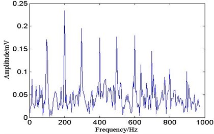
Fig. 11Envelope spectrum of no processed with spatial correlation
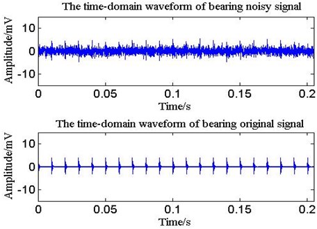
From the Fig. 13 it is the waveform of bearing inner fault signals and the one denoised by spatial correlation. Because of the influence of the noise, the fault features of inner ring fault signal are not obvious. After being denoised by spatial correlation, the inner race fault vibration signals’ noise is decreased obviously, and the impact of the waveform is more clear.
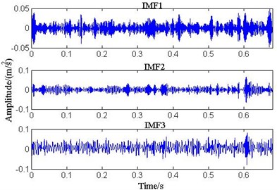
In Fig. 14, the signals are processed by ALIFD. And IMF3 (the stronger correlation) is analyzed by the envelope demodulation in Fig. 15.
Fig. 12The schematic diagram of experimental device
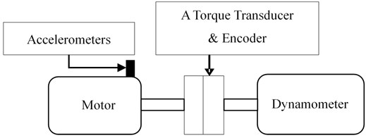
Fig. 13The waveform of bearing vibration signal
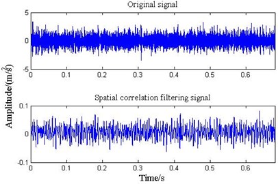
Fig. 14Time-domain waveform of ALIFD
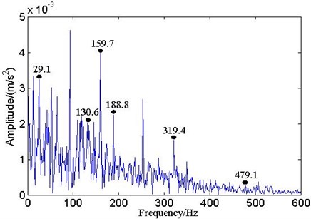
In Fig. 15, the vibration signals of the bearing inner race fault include the BPFI and harmonics, sidebands spaced at . Based on the synthetic analysis of the spatial correlation and ALIFD, bearing inner race weak fault can be diagnosed, and the results are consistent with practice. In order to highlight the advantages of this method, in reference [16] (square envelope spectrum, cepstrum prewhitening, benchmark method), three methods using the same bearing data could not recognize the bearing fault feature (Without repeating the exposition owing to space constraints). Hence, the bearing fault diagnosis based on the spatial correlation and ALIFD is of innovation and practical significance.
Fig. 15The envelope spectrum of IMF3
6. Conclusions
Spatial correlation can use performance characteristics between the real signal and noise on different scales, keep signal details at the same time, effectively reduce noise, and improve the SNR. Simulation shows that this method has obvious advantages over the wavelet threshold denoising. ALIFD is a new adaptive time-frequency method analyzed the nonlinear and non-stationary signals, and remains locality, adaptability and stability. Simulation shows that ALIFD not only overcomes IFD non-adaptability and further improves the smoothness of IFD decomposed component, but also surmounts the presence of spurious modes and residual noise in modes compared with EMD. This paper goes on the bearing inner ring fault as the object, researching the vibration signal denoised by spatial correlation and decomposed into several modes by ALIFD. The simulating signal analysis and bearing fault simulator show that this method based on Spatial Correlation and ALIFD can be available for separating different frequencies of bearing fault vibration signals.
References
-
Sun M. D., Wang H., Liu P. A sparse stacked denoising autoencoder with optimized transfer learning applied to the fault diagnosis of rolling bearings. Measurement, Vol. 146, 2019, p. 305-314.
-
Giv H. H. Directional short-time Fourier transform. Journal of Mathematical Analysis and Applications, Vol. 399, Issue 1, 2013, p. 100-107.
-
Jedlinski L. Multi-channel registered data denoising using wavelet transform, gear parameter identification in a wind turbine gearbox using vibration signals. Eksploatacja i Niezawodnosc-Maintenance and Reliability, Vol. 14, Issue 2, 2012, p. 145-149.
-
Figlus T. A method for diagnosing gearboxes of means of transport using multi-stage filtering and entropy. Entropy, Vol. 21, Issue 5, 2019, p. 2441.
-
Borghesani P., Pennacchi P., Randall R. B., Sawalhi N., et al. Application of cepstrum pre-whitening for the diagnosis of bearing faults under variable speed conditions. Mechanical Systems and Signal Processing, Vol. 36, Issue 2, 2013, p. 370-384.
-
Dybala J. Diagnosing of rolling-element bearings using amplitude level-based decomposition of machine vibration signal. Measurement, Vol. 126, 2018, p. 143-155.
-
Figlus T., Stanczyk M. A method for detecting damage to rolling bearings in toothed gears of processing lines. Metalurgija, Vol. 55, Issue 1, 2016, p. 75-78.
-
Ren Y., Li W., Zhu Z. C., et al. ISVD-based in-band noise reduction approach combined with envelope order analysis for rolling bearing vibration monitoring under varying speed conditions. IEEE Access, Vol. 7, 2019, p. 32072-32084.
-
Xia J. Z., Zhao L., Bai Y. C., et al. Feature extraction for rolling element bearing weak fault based on MCKD and VMD. Journal of Vibration and Shock, Vol. 36, 2017, p. 78-83.
-
Zhao L., Xia J. Z., Wang H., et al. Application of empirical mode decomposition in rolling bearing fault diagnosis. Journal of Military Transportation University, Vol. 18, 2016, p. 49-53.
-
Lin L., Wang Y., Zhou H. M. Iterative filtering as an alternative algorithm for empirical mode decomposition. Advances in Adaptive Data Analysis, Vol. 1, 2009, p. 543-560.
-
Cicona A., Liu J., Zhou H. Adaptive local iterative filtering for signal decomposition and instantaneous frequency analysis. Applied and Computational Harmonic Analysis, Vol. 41, 2016, p. 384-411.
-
Xu Y. Wavelet transform domain filters: a spatially selective noise filtration technique. IEEE Trans Image Processing, Vol. 3, 1994, p. 747-758.
-
Ma Q., Liu Y. Noise reduction method of radar echo signal based on spatial correlation filtering. Fire Control and Command Control, Vol. 41, 2016, p. 113-116.
-
Case Western Reserve University Bearing Data Center, http://csegroups.case.edu/ bearingdatacenter/home.
-
Smith W. A., Randall R. B. Rolling element bearing diagnostics using the Case Western Reserve University data: A benchmark study. Mechanical Systems and Signal Processing, Vol. 64, 2015, p. 100-131.
About this article

This work was supported by the National Natural Science Foundation of China (No. 41631072; 41774021), the Hubei Province Natural Science Foundation of China (No. 2017CFB672).
