Fault diagnosis of rolling bearings based on improved enhanced envelope spectrum

Huang, Baoyu; Zhang, Yongxiang; Zhu, Danchen

doi:10.21595/jve.2020.21668

Journal of Vibroengineering

Browse Journal

Submit article

Published: 04 February 2021

Check for updates

Fault diagnosis of rolling bearings based on improved enhanced envelope spectrum

Baoyu Huang¹

Yongxiang Zhang²

Danchen Zhu³

^{1, 2}Department of Power Engineering, Naval University of Engineering, Wuhan, China

³Department of Mechanical and Electrical Engineering, Naval Petty Officer Academy, Bengbu, China

Corresponding Author:

Yongxiang Zhang

Cite the article Download PDF

Downloads 1066

WoS Core Citations 2

CrossRef Citations 2

Abstract

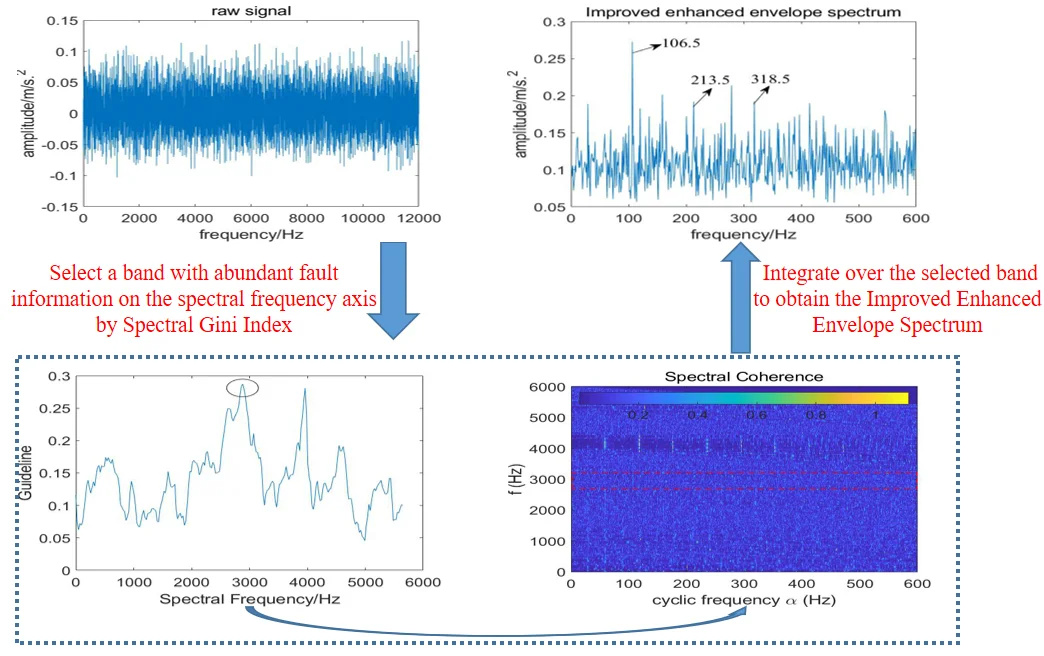
Aiming at the problem that traditional fast spectral correlation (Fast-SC) cannot effectively extract the fault feature of rolling bearings under strong background noise, we propose to select a band with abundant fault information on the spectral frequency axis by Spectral Gini Index (SGI) and integrate over them to obtain the Improved Enhanced Envelope Spectrum (IEES). The proposed method doesn’t rely on the selection of precise fault characteristic frequency, and has a good industrial application prospect. The simulated and experimental results of rolling bearings prove the effectiveness of the algorithm.

Fault diagnosis of rolling bearings based on improved enhanced envelope spectrum

Highlights

Selecting an appropriate integration interval could enhance the fault feature extraction capability of Fast-SC
Compared with kurtosis, Spectral Gini Index is more robust, so it is applied for selecting the optimal integration interval
Compared with Improved Envelope Spectrum by Alpha Maximization (IESAM), the proposed algorithm doesn’t rely on the selection of precise fault characteristic frequency and has a better industrial application prospect
Simulated and experimental signal indicate that the proposed algorithm performs better than the algorithm based on resonance demodulation and Spectral Gini Index

1. Introduction

Rolling bearings have been widely used as one of the important parts of rotating machinery, and their operating status directly affects the performance of the whole machine. Therefore, condition monitoring and fault diagnosis for rolling bearings are particularly necessary. However, due to the complexity of mechanical equipment, cyclostationary signals generated by early bearing defects are often submerged in strong background noise, and the measured vibration signals are usually non-stationary and nonlinear, which greatly increase the difficulty of rolling bearings’ fault feature extraction.

Time domain analysis [1, 2] is the earliest technology used for rolling bearings’ fault diagnosis. It utilizes the basic digital and statistical characteristics of vibration signals to analyze the signal. However, it heavily relies on the experience of analysts. Spectrum analysis [3, 4] is the description of the original signal distribution in the frequency domain, it can provide more intuitive characteristic information than the time-domain waveform. But, owing to the non-stationarity and non-linearity of the measured vibration signal, the applications of the above methods are restricted. So, methods based on time-frequency analysis [5-7] and AI technology [8-10] are developing rapidly in these years and have achieved great success. Whereas, AI-based technologies usually require abundant of data and often run for a long time, which undoubtedly limit the applications of such algorithms. In contrast, time-frequency analysis technology is much more convenient.

As one of the time-frequency analysis techniques, resonance demodulation has been widely used because of its simplicity and effectiveness. When the faulty bearing is operating, the system will resonate. Therefore, how to find the resonance frequency band of the signal becomes the key to the fault diagnosis of the rolling bearings. However, strong background noise such as impulse electromagnetic noise and periodic harmonic noise generated by shaft rotation etc. has great influence on the selection of the resonance frequency band [11]. To solve the problem, Antoni [12] proposed Fast Kurtogram based on maximum kurtosis, Wang et al. [13] combined ensemble local mean decomposition and Fast Kurtogram to extract the fault features of rolling bearings. However, when the non-Gaussian noise in the signal is strong or the fault period is shorter than the response time of a single pulse due to the high speed of rolling bearings, Fast Kurtogram cannot achieve a great demodulation effect [14]. To take the cyclic periodicity of the fault features into account, McDonald et al. [15] proposed to find the resonance frequency band by maximum correlated kurtosis; Zhang et al. [16] used flexible analytical wavelet transform to filter the vibration signal adaptively, then windowed correlated kurtosis was conducted on the filtered signals to isolate each fault mode, experimental results proved its effectiveness. However, algorithms based on correlated kurtosis rely on the selection of precise fault characteristic frequency, which limits their applications.

Gini index was originally used to measure the inequality of economic wealth. It has recently been applied to the field of fault diagnosis and has achieved great success [17]. Miao et al. [18] used Gini index instead of kurtosis to select the resonance frequency band, results showed that Gini index was more robust; Muhammad N. Albezzawy et al. [19] introduced Gini index into the MED, AR model and Morlet wavelet filtering, and the combination of them was successfully applied to the fault diagnosis of rolling bearings; On the basis of the Gini index, Wang et al. [20] proposed the spectral Gini index and applied it to Fast Kurtogram, Compared with the traditional Fast Kurtogram, results showed that spectral Gini index is more suitable for the fault diagnosis of rolling bearings.

In addition to the algorithms based on resonance demodulation, spectral correlation analysis also plays an important role on the fault diagnosis of rolling bearings. However, it is difficult to directly calculate the spectral correlation of the signal, so averaged cyclic periodogram [21], cyclic modulation spectrum [22] and Fast-SC [23] was proposed to calculate the spectral correlation of the signal in succession. Among them, Fast-SC has been widely used due to its efficiency and accuracy. Moreover, Antoni integrated over the full band of spectral frequencies to obtain Enhanced Envelope Spectrum (EES). Zhu et al. [24] combined Fast-SC and Teager-Kaiser energy operator to extract the fault features of rolling bearings under variable speed. However, the traditional EES retains too much noise component in the signal, which is not conducive to the fault diagnosis of rolling bearings under strong background noise; Tang et al. [25] preprocessed the signal with singular negentropy difference spectrum firstly, then analyzed the denoised signal by Fast-SC and obtained its fourth-order energy Spectrum, finally determined the best integration interval of the signal by observation. Simulated and experimental results indicated its effectiveness. However, the algorithm proposed by Tang still needs to determine the integration interval through our own observation, while when the background noise is too strong, it is difficult to select a suitable integration interval through artificial observation. Alexandre Mauricio et al. [26] proposed to utilize alpha maximization to improve the enhanced envelope spectrum, but it relied on the selection of accurate fault characteristic frequency, which is usually difficult in the measured signal due to speed fluctuations or rolling element slippage.

To solve the above problems, while considering the robustness of the spectral Gini index and the powerful fault feature extraction capability of Fast-SC, the idea of resonance demodulation is introduced into Fast-SC in this paper. Firstly, the signal is analyzed by Fast-SC; then, the bandwidth of integration interval is fixed and spectral Gini index of the signal under different integration intervals is calculated; finally, the integration interval with the largest spectral Gini index is selected, then the corresponding enhanced envelope spectrum can be obtained.

2. Basic principles

2.1. Fast-SC

Spectral correlation is a function of the spectral frequency $f$ and the cyclic frequency $α$ . Since the bearing fault signal can be described as a second-order cyclostationary signal, it can be defined as:

1

R_{x} (t, τ) = R_{x} (t + T, τ) = E \{x (t) x {(t - τ)}^{*}\},

where, $R_{x}$ stands for the auto-correlation function, $E$ is the ensemble average operator, $x (.)$ is the signal, $t$ stands for time variable, $T$ is the fault period and $τ$ represents the time delay. Based on Eq. (1), spectral correlation can be defined as:

2

S_{x} (α, f) = \underset{W \to \infty}{l i m} \frac{1}{W} E \{X_{W}^{*} (f) X_{W} (f + α)\},

where $X_{W} (f) = \int_{- W / 2}^{+ W / 2} x (t) e^{- j 2 π f t} d t$ is the Fourier transform of the signal $x (t)$ over a time interval $W$ , and the spectral coherence of the signal can be obtained by normalizing the spectral correlation:

3

γ_{x} (α, f) = \frac{S_{x} (α, f)}{\sqrt{S_{x} (0, f - α / 2) S_{x} (0, f + α / 2)}},

where, $γ_{x} (α, f)$ is the spectral coherence of the signal.

On this basis, Antoni [23] further proposed Enhanced Envelope Spectrum (EES), which is to integrate the spectral coherence $γ_{x} (α, f)$ over the full frequency, the expression is as follow:

4

S_{E E S} (α) = \frac{1}{f_{s} / 2} \int_{0}^{f_{s} / 2} |γ (α, f)| d f,

where, $f_{s}$ is the sampling frequency.

However, integrating spectral coherence of the signal over the full frequency band will introduce excessive noise interference, which will affect the extraction of fault features. Therefore, it is necessary to select a suitable integration interval to minimize the interference of noise components, and we propose to select the optimal integration interval based on spectral Gini index due to its robustness.

2.2. Spectral Gini index

Gini index was first proposed by Corrado Gini [27] to measure the inequality of society and economic wealth, it is essentially a sparsity index. Niall Hurley pointed out that the concentration of signal’s energy is proportional to its sparsity [28]. Meanwhile, the energy of the resonance frequency band which contains the most abundant fault information in the fault signal appears the most concentrated, so the resonance frequency band appears the sparsest. Based on this characteristic, Gini index can be utilized in the field of fault diagnosis of rolling bearings. Given $x = [x (1), x (2), \dots, x (N)]$ , and rearrange them in ascending order $|x_{[1]}| \leq |x_{[2]}| \leq \dots \leq |x_{[N]}|$ , then Gini index can be calculated as:

5

G I (x) = 1 - 2 \sum_{k = 1}^{N} \frac{|x_{[k]}|}{{‖x‖}_{1}} \times (\frac{N - k + 0.5}{N}),

where, ${‖x‖}_{1}$ is the $l_{1}$ norm of $x$ , $k$ is the subscript of x after rearrangement and $N$ is the length of $x$ .

Furthermore, Wang et al. [19] defined spectral Gini index and used it to extract bearings’ fault features:

6

S G I (x) = 1 - 2 \sum_{k = 1}^{N} \frac{S E_{l, h}^{r} [n]}{{‖S E_{l, h}^{r} [n]‖}_{1}} \times (\frac{N - k + 0.5}{N}),

where, $l$ and $h$ are the left and right cutoff frequencies of the band-pass filter, $S E_{l, h} [n]$ represents the squared envelope of the filtered signal, $S E_{l, h}^{r} [n]$ means rearranged $S E_{l, h} [n]$ in ascending order.

2.3. Enhanced envelope spectrum improved by spectral Gini index

Barszcz pointed out that the bandwidth of filter should be no less than 3 times of fault characteristic frequency [29]. So we set the length of the integration interval at 3 times the fault characteristic frequency. Combining with spectral Gini index, we use the following formula to select the optimal integration interval:

7

g (f) = 1 - 2 \sum_{n = 1}^{N} \frac{s o r t_{n} (\sum_{f}^{f + 3 f_{f a u l t}} |γ (α, f)|)}{\sum_{α = f l o o r (0.98 f_{f a u l t})}^{c e i l (1.02 f_{f a u l t})} \sum_{f}^{f + 3 f_{f a u l t}} |γ (α, f)|} * (\frac{N - n + 0.5}{N}),

where, $f_{f a u l t}$ represents theoretical fault characteristic frequency, $s o r t (.)$ means rearranged the data in ascending order. The subscript $n$ indicates the position of the data after reordering, and $N$ indicates the length of the signal. What’s more, $f l o o r (.)$ means rounding down, and $c e i l (.)$ represents rounding up. Taking into account speed fluctuations and rolling element slippage, the actual fault characteristic frequency may have an error with the theoretical value but within 2 %, so the range of cyclic frequency $α$ should be selected as [0.98 $f_{f a u l t}$ , 1.02 $f_{f a u l t}$ ].

The higher the value of $g (f)$ is, the larger the spectral Gini index of the corresponding integration frequency band is, which means the richer fault information it contains, and the easier it is to extract fault features. Therefore, we can determine the optimal integration frequency band by the maximum value of $g (f)$ . The proposed method doesn’t rely on the precise fault characteristic frequency determined in advance, nor does it need to manually find the optimal integration interval, which means it has a good industrial application prospect.

3. Simulation verification

In order to verify the effectiveness of the proposed algorithm, this section constructs a simulated signal of rolling bearings under strong background noise. The model of the simulated signal is as follow:

8

\{\begin{array}{l} x_{1} (t) = \sum_{i = 1}^{N} A_{i} s (t - i T - t_{i}) + B (t) + n (t) + m (t), \\ A_{i} = 4 c o s (2 π f_{r} t + \frac{π}{2}) + 0.5, \\ B (t) = 1.2 c o s (2 π f_{1} t + \frac{π}{2}) + 0.9 c o s (2 π f_{2} t), \\ s (t) = e^{- 2 π f_{n} r t} s i n (2 π f_{n} t), \end{array}

where, $f_{r} =$ 42 Hz represents rotating frequency, $A_{i}$ denotes the amplitude modulation with the cycle of 1/ $f_{r}$ , $f_{n} =$ 3200 Hz is the natural frequency of the system and $r =$ 0.05 represents damping coefficient. $t_{i} =$ 0.01 $T$ -0.02 $T$ denotes the delay caused by the slippage of rolling element in $i$ th cycle. $T =$ 1/185 s represents the period during which the fault occurs, which means the fault characteristic frequency is 185 Hz. The harmonic $B (t)$ is applied to simulate the interference components and the value of $f_{1}$ and $f_{2}$ are 80 Hz and 100 Hz respectively. $m (t)$ represents random impulsive noise, $n (t)$ represents Gaussian noise. The signal-to-noise ratio of this signal is –6.36 dB if no white noise is added, and the ratio is –16.7 dB after adding white noise. The sampling frequency is 32768 Hz and the sampling time is 1 s. Fig. 1 is the time domain waveform of the simulated signal, disturbed by strong background noise, periodic impulses related to the local damage can hardly be observed.

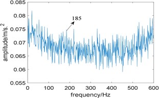
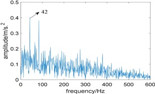
In order to highlight the difficulty of extracting the fault feature of the simulated signal, Fast-SC is utilized to analyze the simulated signal, and the corresponding enhanced envelope spectrum is shown in Fig. 2. Due to the interference of strong background noise, only fault characteristic frequency 185 Hz can be identified vaguely, which means the traditional Fast-SC doesn’t perform well.

Fig. 1Time domain waveform of simulation signal

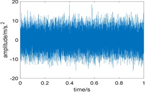
Fig. 2The result of the simulation signal analyzed by Fast-SC

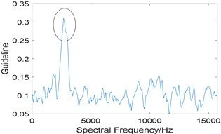
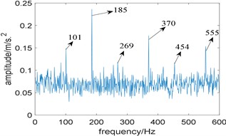
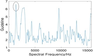
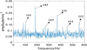
Now, the proposed algorithm is used to analyze the simulated signal, and the window length of STFT (Short Time Fourier Transform) is selected as 512. Due to the limitation of spectral frequency resolution, the length of integration interval is slightly larger than 3 times of fault characteristic frequency, which is taken as 576. The relevant curve is shown as Fig. 3(a), and the integration interval corresponding to the maximum value of $g (f)$ is [2752 3328]. Its corresponding improved enhanced envelope spectrum is shown in Fig. 3(b), where background noise is significantly suppressed, fault characteristic frequency 185 Hz and its harmonics 370 Hz and 555 Hz are prominent. What’s more, sidebands 101 Hz, 269 Hz and 454 Hz modulated by rotating frequency can also be observed too.

Fig. 3Results of the proposed method: a) the curve of gf; b) corresponding improved enhanced envelope spectrum

a)

b)

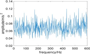
In addition, kurtosis is utilized to select the optimal integration interval, and the length of integration interval is also set as 576. Fig. 4(a) shows the relationship between kurtosis and integration interval, where several points have a high value of kurtosis, which indicates that kurtosis is less robust than spectral Gini index. It is worth noting that in the integration interval [2752 3328], kurtosis also has a peak value. However, the optimal integration interval selected by kurtosis is [1344 1920], and its corresponding enhanced envelope spectrum is shown in Fig. 4(b). Due to the interference of strong background noise, fault characteristic frequency and its harmonies cannot be identified, which means the algorithm based on Fast-SC and kurtosis fails to extract the fault feature.

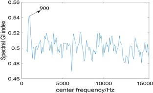
In order to further highlight the superiority of the proposed algorithm, the algorithm based on traditional resonance demodulation and spectral Gini index is applied to analyze the simulated signal. The bandwidth is also fixed at 3 times the fault characteristic frequency. Fig. 5(a) shows the relationship between spectral Gini index and center frequency, and the optimal center frequency selected by the algorithm is 900 Hz; its corresponding squared envelope spectrum is shown in Fig. 5(b), where 42 Hz is rotating frequency, and no fault feature can be identified.

Fig. 4Results of the algorithm based on Fast-SC and kurtosis: a) the relationship between kurtosis and integration interval; b) corresponding improved enhanced envelope spectrum

Results of the algorithm based on Fast-SC and kurtosis: a) the relationship between kurtosis and integration interval; b) corresponding improved enhanced envelope spectrum

a)

b)

Fig. 5Results of the algorithm based on traditional resonance demodulation and spectral Gini index: a) The relationship between spectral Gini index and center frequency, b) corresponding squared envelope spectrum

Results of the algorithm based on traditional resonance demodulation and spectral Gini index: a) The relationship between spectral Gini index and center frequency, b) corresponding squared envelope spectrum

a)

b)

What’s more, the algorithm named Improved Envelope Spectrum by Alpha Maximization (IESAM) proposed in the literature [26] is also used for comparison, the algorithm is described as follow:

9

\{\begin{array}{l} S D_{A M} (f) = \prod_{i = 1}^{k} γ (i \times α_{f a u l t}, f), \\ m a x (S D_{A M} (f)) * t h r e s = S D_{A M} (f_{1}) = S D_{A M} (f_{2}), f_{1} < f_{m a x} < f_{2}, \\ S_{I E S} (α) = \frac{1}{f_{2} - f_{1}} \int_{f_{1}}^{f_{2}} |γ (α, f)| d f, \end{array}

where, $S D_{A M} (f)$ is used to select the integral frequency band with the most obvious fault features, $t h r e s =$ 0.7 is the threshold parameter, $f_{m a x}$ is the frequency corresponding to the maximum value of $S D_{A M} (f)$ , and $α_{f a u l t}$ represents the fault characteristic frequency.

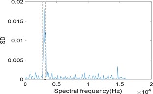
Fig. 6Results of the simulation signal analyzed by IESAM when αfault= 185 Hz: a) the relationship between SD and integration interval; b) corresponding enhanced envelope spectrum

Results of the simulation signal analyzed by IESAM when αfault= 185 Hz: a) the relationship between SD and integration interval; b) corresponding enhanced envelope spectrum

a)

b)

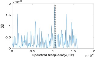
Fig. 7Results of the simulation signal analyzed by IESAM when αfault= 184 Hz: a) the relationship between SD and integration interval; b) corresponding enhanced envelope spectrum

Results of the simulation signal analyzed by IESAM when αfault= 184 Hz: a) the relationship between SD and integration interval; b) corresponding enhanced envelope spectrum

a)

b)

To prove that the effectiveness of IESAM depends on the precise selection of fault characteristic frequency, we choose $α_{f a u l t} =$ 185 Hz and $α_{f a u l t} =$ 184 Hz respectively for comparison, and $k$ is both taken as 3. Fig. 6(a) shows the curve of $S D_{A M} (f)$ when $α_{f a u l t} =$ 185 Hz, and the selected integration interval is [2880 3136], which is close to the integration interval selected in Fig. 3(a). Fig. 6(b) is the corresponding enhanced envelope spectrum of the selected integration interval, from which we can see that noise components have been effectively suppressed, fault characteristic frequency 185 Hz and its harmonies 370 Hz and 555 Hz can be identified clearly, what is more, sidebands 101 Hz, 269 Hz and 454 Hz modulated by rotating frequency can be observed too. Comparing Fig. 3(b) with Fig. 6(b), both perform well. Fig. 7(a) is the curve of $S D_{A M} (f)$ when $α_{f a u l t} =$ 184 Hz, and the selected integration interval is [10304 10560]. Fig. 7(b) is the enhanced envelope spectrum of the selected integration interval. Due to the interference of strong background noise, fault characteristic frequency and its harmonies cannot be identified. Comparing Fig. 6 with Fig. 7, we conclude that the effectiveness of IESAM depends heavily on the correct selection of fault characteristic frequency, which restricts the application of this method in industry. In contrast, the algorithm proposed in this paper does not rely on the actual fault characteristic frequency determined in advance and has a wider application prospect.

4. Experimental verification

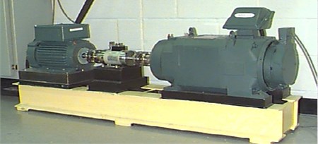
Data used in this paper is obtained from the Case Western Reserve University Bearing Data Center database [30]. The experimental test rig (shown in Fig. 8) is comprised of a 2-hp motor, a torque sensor/encoder, a power meter, accelerometers, and electronic control unit. The drive end motor shaft is supported by deep groove ball bearing (JEM SKF 6205-2RS) which contains outer race fault generated by electro-discharge machining, and the fault diameter is 0.3556 mm. The outer diameter of the bearing is 52 mm and the inner diameter is 25 mm, the rolling element diameter is 8 mm, the number of rolling elements is 9, and the contact angle is 0°. The fault data used in this paper is 198 mat whose sampling frequency is 12000 Hz and the test speed is 1772 r/min. In order to reduce calculation time, we only take 12000 points for analyzed, and the theoretical fault characteristic frequency is calculated as 105.87 Hz.

Fig. 8The test rig

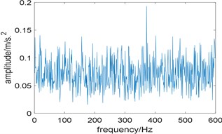
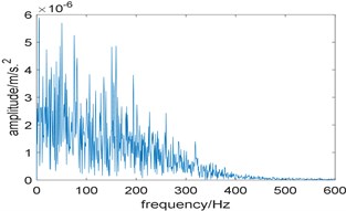
Now we use Fast-SC to analyze the signal and the result is shown in Fig. 9. Due to the interference of strong background noise, the spectral line of 106.5 Hz which is close to the theoretical fault characteristic frequency is faintly visible, and its harmonies cannot be identified. What’s more, the frequency of 29.24 Hz represents rotating frequency and 118 Hz is one of its harmony. So, we come to the conclusion that the performance of Fast-SC is not ideal.

Fig. 9Result of the experimental signal analyzed by Fast-SC

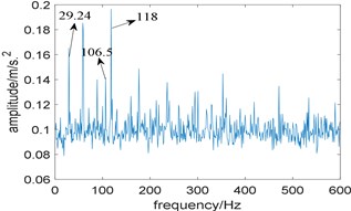
Fig. 10Results of the proposed algorithm: a) the curve of gf; b) corresponding improved enhanced envelope spectrum

a)

b)

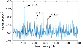
Then, the proposed algorithm is applied to analyze the experimental signal, the window length of STFT is choose as 512 and the length of the integration interval is selected as 351, which is slightly larger than 3 times of fault characteristic frequency due to the limitation of the spectral frequency resolution. Fig. 10(a) shows the relationship between the value of $g (f)$ and integration interval, from which the optimal integration interval is selected as [2883 3234]; Fig. 10(b) is the corresponding improved enhanced envelope spectrum, where fault characteristic frequency 106.5 Hz and its harmonies 213.1 Hz and 318.5 Hz can be identified. Comparing Fig. 10(b) with Fig. 9, we come to the conclusion that the proposed algorithm can suppress the noise components obviously and has the stronger capability to extract the fault feature.

Fig. 11Results of the algorithm based on Fast-SC and kurtosis: a) the relationship between kurtosis and integration interval; b) corresponding improved enhanced envelope spectrum

a)

b)

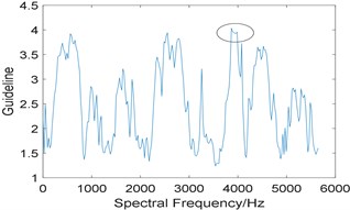
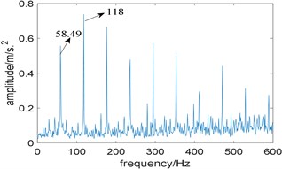
In addition, kurtosis is utilized to select the optimal integration interval. Fig. 11(a) shows the relationship between kurtosis and integration interval, where several points have a high value of kurtosis, which indicates that kurtosis is sensitive to background noise. It is worth noting that the kurtosis is also very large at the interval [2789 3140], but the integration interval corresponding to the maximum kurtosis is [3867 4218]. Fig. 11(b) is the enhanced envelope spectrum under the corresponding integration interval, where 58.49 Hz represents the double of rotating frequency, and there is no useful information can be extracted.

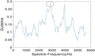
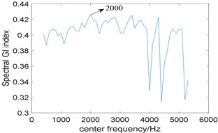
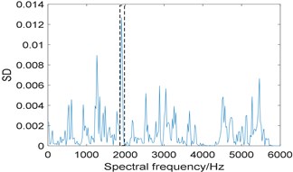
In order to further highlight the superiority of the proposed algorithm, the method based on traditional resonance demodulation and spectral Gini index is applied to analyze the experimental signal, and the bandwidth is fixed at 3 times the fault characteristic frequency. Fig. 12(a) shows the relationship between spectral Gini index and center frequency, the optimal center frequency is selected as 2000 Hz; its corresponding squared envelope spectrum is shown in Fig. 12(b), due to the influence of strong background noise, there is no useful information can be extracted, which means the method does not perform well. Comparing Fig. 10(b) with Fig. 12(b), the proposed algorithm has stronger fault feature extraction capability.

Fig. 12Results of the method based on traditional resonance demodulation and spectral Gini index: a) the relationship between spectral Gini index and center frequency; b) corresponding squared envelope spectrum

Results of the method based on traditional resonance demodulation and spectral Gini index: a) the relationship between spectral Gini index and center frequency; b) corresponding squared envelope spectrum

a)

b)

Fig. 13Results of the experimental signal analysed by IESAM when αfault= 105.5 Hz: a) the relationship between SD and integration interval; b) corresponding enhanced envelope spectrum

Results of the experimental signal analysed by IESAM when αfault= 105.5 Hz: a) the relationship between SD and integration interval; b) corresponding enhanced envelope spectrum

a)

b)

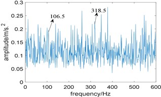
Then, IESAM is applied to analyze the experimental signal, the window length of STFT is choose as 512, $α_{f a u l t}$ is selected as 105.5 Hz, which is closest to the theoretical value, and $k$ is taken as 3. Fig. 13(a) is the curve of $S D_{A M} (f)$ , where the optimal integration interval is selected as [1852 1969]; Fig. 13(b) is the corresponding enhanced envelope spectrum, due to the interference of strong background noise, fault characteristic frequency 106.5 Hz and one of its harmonies 318.5 Hz is faintly visible, comparing Fig. 10(b) with Fig. 13(b), the proposed algorithm performs better.

What’s more, Mantas Landauskas et al. [31] combined permutation entropy and convolutional neural network for bearings’ fault classification, and the data was obtained from the Case Western Reserve University Bearing Data Center database too. Results showed that the classification accuracy of outer ring fault data when the defect is on drive end (sampled at 12k) was 0.779, which was not high enough. Wade A. Smith et al. [32] further pointed out that the data used in the paper was difficult to be analyzed. However, the proposed algorithm can extract the fault feature effectively, which represents the superiority of the algorithm.

5. Conclusions

From the analyses of simulated signal and experimental signal, we conclude that the proposed algorithm based on Fast-SC and spectral Gini index can extract fault features of rolling bearings effectively, and have the following conclusions:

1) In actual engineering, strong background noise as well as the deviation of the actual fault characteristic frequency from the theoretical value caused by speed fluctuations or rolling element slippage will increase the difficulty of extracting fault features of the rolling bearings.

2) We use spectral Gini index and the kurtosis to select the optimal integration interval, results show that spectral Gini index is more robust than kurtosis. What is more, results of simulated and experimental signal indicate that the proposed algorithm performs better than the algorithm based on resonance demodulation and spectral Gini index.

3) The proposed algorithm is also compared with IESAM and traditional Fast-SC. Results show that the effectiveness of IESAM highly depends on the precise selection of fault characteristic frequency, while traditional Fast-SC will introduce excessive background noise, which is not conducive to the extraction of fault features. In contrast, the proposed algorithm does not rely on the precise selection of fault characteristic frequency, and the selection of the optimal integration interval can filter out the interference of background noise effectively. So, it has stronger fault feature extraction capability and has a good industrial application prospect.

References

Grządziela A. A., Musiał J. B., Muślewski L. B., et al. A method for identification of non-coaxiality in engine shaft lines of a selected type of naval ships. Polish Maritime Research, Vol. 22, Issue 1, 2015, p. 65-71.

Publisher
Shengli Zhang, Tang J. Integrating angle-frequency domain synchronous averaging technique with feature extraction for gear fault diagnosis. Mechanical Systems and Signal Processing, Vol. 99, 2018, p. 711-729.

Publisher
Randall R. B., Antoni J., Smith W. A. A survey of the application of the cepstrum to structural modal analysis. Mechanical Systems and Signal Processing, Vol. 118, 2019, p. 716-741.

Publisher
Zamani M., Hajesmaeili H. N., Zandi M. H. Amplitude-cyclic frequency decomposition of vibration signals for bearing fault diagnosis based on phase editing. Mechanical Systems and Signal Processing, Vol. 103, 2018, p. 76-88.

Publisher
Qin Chao-Ren, Wang Dong-Dong, Xu Zhi, et al. Improved empirical wavelet transform for compound weak bearing fault diagnosis with acoustic signals. Applied Sciences, Vol. 10, Issue 2, 2020, p. 1-16.

Publisher
Wang Jun, Du Gui-Fu, Zhu Zhong-Kui, et al. Fault diagnosis of rotating machines based on the EMD manifold. Mechanical Systems and Signal Processing, Vol. 135, 2020, p. 106443.

Publisher
Ding Jia-Kai, Huang Liang-Pei, Xiao Dong-Ming, et al. GMPSO-VMD algorithm and its application to rolling bearing fault feature extraction. Sensors, Vol. 20, Issue 7, 2020, p. 1946.

Publisher
Kolar Davor, Lisjak Dragutin, Pająk Michał, et al. Fault diagnosis of rotary machines using deep convolutional neural network with wide three axis vibration signal input. Sensors, Vol. 20, Issue 14, 2020, p. E4017.

Publisher
Pająk Michał, Muślewski Łukasz, Landowski Bogdan, et al. Fuzzy identification of the reliability state of the mine detecting ship propulsion system. Polish Maritime Research, Vol. 26, Issue 1, 2019, p. 55-64.

Publisher
Spyridon Plakias, Yiannis Boutalis S. Fault detection and identification of rolling element bearings with attentive dense CNN. Neurocomputing, Vol. 405, 2020, p. 208-217.

Publisher
Miao Yong-Hao, Zhao Ming, Lin Jing Identification of mechanical compound-fault based on the improved parameter-adaptive variational mode decomposition. ISA Transactions, Vol. 84, 2019, p. 108-124.

Publisher
Antoni J. Fast computation of the kurtogram for the detection of transient faults. Mechanical Systems and Signal Processing, Vol. 21, Issue 1, 2005, p. 108-124.

Publisher
Wang Lei, Liu Zhi-Wen, Miao Qiang, et al. Time-frequency analysis based on ensemble local mean decomposition and fast kurtogram for rotating machinery fault diagnosis. Mechanical Systems and Signal Processing, Vol. 103, 2018, p. 60-75.

Publisher
Abboud D. A., Elbadaoui M. A., Smith W. A., et al. Advanced bearing diagnostics: a comparative study of two powerful approaches. Mechanical Systems and Signal Processing, Vol. 114, 2019, p. 604-627.

Publisher
McDonald G. L., Zhao Qing, Zuo M. J. Maximum correlated Kurtosis deconvolution and application on gear tooth chip fault detection. Mechanical Systems and Signal Processing, Vol. 33, 2012, p. 237-255.

Publisher
Zhang Chun-Lin, Liu Yu-Ling, Wan Fang-Yi, et al. Adaptive filtering enhanced windowed correlated kurtosis for multiple faults diagnosis of locomotive bearings. ISA Transactions, Vol. 101, 2020, p. 421-429.

Publisher
Janssens O., Loccufier M., Van De Walle R., et al. Data-driven imbalance and hard particle detection in rotating machinery using infrared thermal imaging. Infrared Physics and Technology, Vol. 82, 2017, p. 28-39.

Publisher
Miao Yong-Hao, Zhao Ming, Lin Jing Improvement of kurtosis-guided-grams via Gini index for bearing fault feature identification. Measurement Science and Technology, Vol. 28, Issue 12, 2017, p. 125001.

Publisher
Muhammad Albezzawy N., Mohamed Nassef G., Nader Sawalhi Rolling element bearing fault identification using a novel three-step adaptive and automated filtration scheme based on Gini index. ISA Transactions, Vol. 101, 2020, p. 453-460.

Publisher
Wang Dong Some further thoughts about spectral kurtosis, spectral L2/L1 norm, spectral smoothness index and spectral Gini index for characterizing repetitive transients. Mechanical Systems and Signal Processing, Vol. 108, 2018, p. 58-72.

Publisher
Antoni J. Cyclic spectral analysis in practice, Mechanical Systems and Signal Processing, Vol. 21, Issue 2, 2007, p. 597-630.

Publisher
Antoni J., Hanson D. Detection of surface ships from interception of cyclostationary signature with the cyclic modulation coherence. IEEE Journal of Oceanic Engineering, Vol. 37, Issue 3, 2012, p. 478-493.

Publisher
Antoni J., Ge Xin, Hamzaoui N. Fast computation of the spectral correlation. Mechanical Systems and Signal Processing, Vol. 92, 2017, p. 248-277.

Publisher
Zhu Dan-Chen, Zhang Yong-Xiang, Zhu Qun-Wei Fault diagnosis method for rolling element bearings under variable speed based on TKEO and Fast-SC. Journal of Failure Analysis and Prevention, Vol. 18, Issue 1, 2018, p. 2-7.

Publisher
Tang Gui Ji, Tian Tian Compound fault diagnosis of rolling bearing based on singular negentropy difference spectrum and integrated fast spectral correlation. Entropy, Vol. 22, Issue 3, 2020, p. 367.

Publisher
Alexandre Mauricio, Qi Jun-Yu, Wade Smith A. C. Bearing diagnostics under strong electromagnetic interference based on integrated spectral coherence. Mechanical Systems and Signal Processing, Vol. 140, 2020, p. 106673.

Publisher
Gini C. Measurement of inequality of incomes. The Economic Journal, Vol. 31, Issue 121, 1921, p. 124-136.

Publisher
Hurley N., Rickard S. Comparing measures of sparsity. IEEE Transactions on Information Theory, Vol. 55, Issue 10, 2009, p. 4723-4741.

Publisher
T. Barszcz Jabłoński. A novel method for the optimal band selection for vibration signal demodulation and comparison with the kurtogram. Mechanical Systems and Signal Processing, Vol. 25, Issue 1, 2011, p. 431-451.

Publisher
Case western reserve university bearing data center website. https://csegroups.case.edu/ bearingdatacenter/ home.

Search CrossRef
Mantas Landauskas, Maosen Cao, Minvydas Ragulskis. Permutation entropy-based 2D feature extraction for bearing fault diagnosis. Nonlinear Dynamics, Vol. 102, Issue 3, 2020, p. 1717-1731.

Publisher
Smith W. A., Randall R. B. Rolling element bearing diagnostics using the Case Western Reserve University data: a benchmark study. Mechanical Systems and Signal Processing, Vol. 64, 2015, p. 100-131.

Publisher

Cited by

Weighted envelope spectrum based on reselection mechanism and its application in bearing fault diagnosis

Yongxiang Zhang | Baoyu Huang

(2023)

A novel spectral coherence-based envelope spectrum for railway axle-box bearing damage identification

Bingyan Chen | Dongli Song | Weihua Zhang | Yao Cheng

(2023)

About this article

Received

20 August 2020

Accepted

31 December 2020

Published

04 February 2021

SUBJECTS

Fault diagnosis based on vibration signal analysis

DOI

https://doi.org/10.21595/jve.2020.21668

Keywords

rolling bearing

fault diagnosis

fast spectral correlation

spectral Gini index

This is an open access article distributed under the Creative Commons Attribution License, which permits unrestricted use, distribution, and reproduction in any medium, provided the original work is properly cited.

Previous article in issue Previous Next article in issue Next

Research article

2024 02 18

Rolling bearing compound fault diagnosis based on spatiotemporal intrinsic mode decomposition

Zhixing Li, Yuanxiu Zhang, Yanxue Wang

Research article

2023 10 09

Extraction and diagnosis of rolling bearing fault signals based on improved wavelet transform

Zhiqing Cheng

Research article

2022 05 15

The enhancement of fault detection for rolling bearing via optimized VMD and TQWT based sparse code shrinkage

Xing Yuan, Huijie Zhang, Hui Liu

Research article

2021 02 04

Research on fault diagnosis of rolling bearings based on conditional variance statistic and cross-correlation spectrum

Baoyu Huang, Yongxiang Zhang, Danchen Zhu

B. Huang, Y. Zhang, and D. Zhu, “Fault diagnosis of rolling bearings based on improved enhanced envelope spectrum,” Journal of Vibroengineering, Vol. 23, No. 2, pp. 373–384, Feb. 2021, https://doi.org/10.21595/jve.2020.21668

Copy Extrica

Copied to clipboard!

TY  - JOUR
DO  - 10.21595/jve.2020.21668
UR  - https://doi.org/10.21595/jve.2020.21668
TI  - Fault diagnosis of rolling bearings based on improved enhanced envelope spectrum
T2  - Journal of Vibroengineering
AU  - Zhang, Yongxiang
AU  - Huang, Baoyu
AU  - Zhu, Danchen
PY  - 2021
DA  - 2021/02/04
PB  - JVE International Ltd.
SP  - 373-384
IS  - 2
VL  - 23
SN  - 1392-8716
SN  - 2538-8460
ER  - 

Copy Ris

Copied to clipboard!

@article{Zhang_2021,
	doi = {10.21595/jve.2020.21668},
	url = {https://doi.org/10.21595/jve.2020.21668},
	year = 2021,
	month = {feb},
	publisher = {{JVE} International Ltd.},
	volume = {23},
	number = {2},
	pages = {373--384},
	author = {Yongxiang Zhang and Baoyu Huang and Danchen Zhu},
	title = {Fault diagnosis of rolling bearings based on improved enhanced envelope spectrum},
	journal = {Journal of Vibroengineering}
}

Copy Bibtex

Copied to clipboard!

[1]Y. Zhang, B. Huang, and D. Zhu, “Fault diagnosis of rolling bearings based on improved enhanced envelope spectrum,” Journal of Vibroengineering, vol. 23, no. 2, pp. 373–384, Feb. 2021, doi: 10.21595/jve.2020.21668.

Copy IEEE

Copied to clipboard!

Zhang, Yongxiang, Baoyu Huang, and Danchen Zhu. “Fault Diagnosis of Rolling Bearings Based on Improved Enhanced Envelope Spectrum.” Journal of Vibroengineering 23, no. 2 (February 4, 2021): 373–84. https://doi.org/10.21595/jve.2020.21668.

Copy Chicago

Copied to clipboard!

Fault diagnosis of rolling bearings based on improved enhanced envelope spectrum

Abstract

Highlights

1. Introduction

2. Basic principles

2.1. Fast-SC

2.2. Spectral Gini index

2.3. Enhanced envelope spectrum improved by spectral Gini index

3. Simulation verification

4. Experimental verification

5. Conclusions

References

Cited by

About this article

Related Articles