Research on fault diagnosis of rolling bearings based on conditional variance statistic and cross-correlation spectrum

1. Introduction

Rolling bearings are widely used as one of the important parts of rotating machinery, and their operating conditions directly affect the performance of the whole machine. Therefore, condition monitoring and fault diagnosis for rolling bearings are particularly important. Due to the complexity of mechanical equipment and its harsh operating environment, bearing fault signals are often submerged in strong background noise, and the measured vibration signals are usually non-stationary and nonlinear, which greatly increase the difficulty of fault feature extraction of bearing vibration signals.

In order to extract the fault feature of rolling bearings under strong background noise, researchers have proposed many effective methods, such as wavelet transform [1], empirical mode decomposition (EMD) [2], variational mode decomposition (VMD) [3], blind deconvolution algorithm [4-7] and so on. However, strong background noise will interfere with the selection of wavelet basis, which directly affects the effectiveness of wavelet transform; EMD has the problems of end effect and mode mixing, and the algorithm lacks rigorous mathematical reasoning; the performance of VMD depends on the selection of decomposition number and penalty parameter seriously; minimum entropy deconvolution (MED), which aims to restore single dominant pulse, is susceptible to random impulse noise; what’s more, the performance of blind deconvolution algorithm based on the cyclostationarity of fault signal, such as maximum correlated kurtosis deconvolution (MCKD), multipoint optimal minimum entropy deconvolution (MOMEDA) and maximum second-order cyclostationarity blind deconvolution (CYCBD) relies on the selection of fault period, which is usually difficult due to speed fluctuations or rolling element slippage.

Envelope analysis is the most mature method in bearings’ fault diagnosis [8], its performance depends on the correct selection of resonance frequency band. To solve the problem, Antoni proposed Fast Kurtogram to select the resonance frequency band based on the maximum kurtosis [9]. However, the center frequency and bandwidth selected by Fast Kurtogram are not accurate enough, which results in the loss of some useful information, especially under strong non-Gaussian noise, Fast Kurtogram usually fails to extract the fault feature [10]. To solve these problems, Xu et al. [11] constructed a set of filters with variable bandwidth by empirical wavelet transform and obtained a series of empirical modal components, then the optimal empirical mode component was selected according to the maximum kurtosis, simulation and experimental results verified the effectiveness of the method. Based on the cyclostationarity of bearing fault signal, Barszcz et al. [12] proposed protrugram, which fixed the bandwidth and selected the best filter parameters with the maximum squared envelope spectrum kurtosis. However, this method ignores the impulsiveness of the bearing fault signal, which may influence its performance. To alleviate this problem, Antoni took into account the impulsiveness of the fault signal in the time domain and the cyclostationarity in the frequency domain, then proposed infogram [13]. This algorithm calculated the negentropy of squared envelope signal and squared envelope spectrum, then their mean value was used as the objective function to select the optimal frequency band, simulation and experimental results verified its effectiveness. However, under strong impulsive noise, the negentropy of the squared envelope signal may be much larger than that of the squared envelope spectrum, which makes the selected filter band favors impulsiveness more than cyclostationarity [14]. Recently, Gini index which is a measure of sparsity has been used to extract the fault feature of rolling bearings. Miao et al. [15] found that Gini index is more robust to random impulse noise than kurtosis, and used it to select the resonance frequency band. Moreover, he further compared Gini index with kurtosis, results showed that although Gini index is more robust to impulsive noise than kurtosis, its robustness to random white noise is weaker [16].

Justyna et al. [14] performed a short-time Fourier transform on signal and selected the resonance frequency band based on the maximum conditional variance statistic, results showed the feasibility of this algorithm. Then he further compared conditional variance statistic with kurtosis, Gini index, smoothness index and stability index (Alpha selector), results indicated that if the fault signal didn’t contain impulsive noise, all indicators could select the resonant frequency band appropriately, but the method based on the conditional variance statistic performed best; if the fault signal contained strong impulsive noise, only the method based on conditional variance statistic could accurately select the resonant frequency band of the signal [17]. However, the algorithm proposed by Justyna also has the following disadvantages: if the step size is too short, it will affect the calculation efficiency; if the step size is too long, the precise center frequency cannot be selected.

Aiming at the problem that it is difficult to extract the fault feature of rolling bearings under strong background noise, and considering the strong robustness of conditional variance statistic, we propose to optimize the parameters of the filter by conditional variance statistic. What’s more, this paper further researches the effect of bandwidth and center frequency on conditional variance statistic, results show that it can be used as the objective function to select the center frequency but is unreliable to select bandwidth. Fortunately, Barszcz et al. [12] pointed out that bandwidth should be more than three times of fault characteristic frequency. Duan et al. [18] further pointed out that when the bandwidth is $n$ times of fault characteristic frequency, it may also fail to extract $n$ fault related harmonics in the squared envelope spectrum, and proposed that the bandwidth should be slightly greater than four times of fault characteristic frequency. Based on the above considerations, we fix the bandwidth at five times fault characteristic frequency, and choose conditional variance statistic as the objective function, then WOA is utilized to select the optimal center frequency quickly; in order to further suppress the in-band noise, the filtered signal is analyzed by high-order energy operator, and the optimal two energy operators are selected based on FCI for cross-correlation spectrum analysis; finally, the fault feature is extracted by fast Fourier transform.

2. Basic principles

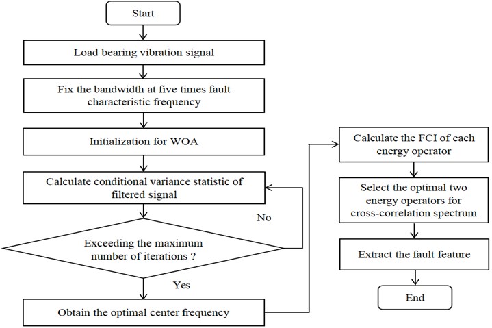
In this section, conditional variance statistic is researched, and results indicate that it can be used as the objective function for selecting the center frequency of the filter, but is not suitable for selecting the bandwidth. Hence, we fix the bandwidth at five times fault characteristic frequency, and WOA is utilized to quickly select the appropriate center frequency; then the filtered signal is analyzed by high-order energy operator analysis; finally, the optimal two energy operators are selected based on FCI for cross-correlation spectrum analysis.

2.1. Selection of the optimal filtering frequency band

2.1.1. Conditional variance statistic

Conditional variance statistic is derived from the statistical phenomenon commonly known as the 20/60/20 rule. Suppose a set of data $Y$ conforms to a Gaussian random distribution, with mean $\alpha$ and standard deviation $\sigma$. ${\mathrm{\Phi }}_{\alpha ,\sigma }$ denotes its distribution function. when 0 $<q<$ 0.5, we can obtain left partitioning $L_q$, right partitioning $R_q$ and middle partitioning $M_q$ of $Y$ using Eq. (1):

1

$\left\{\begin{array}{l}{L}_q=\left(-\infty ,{\varphi }_{a,\sigma }^{-1}\left(q\right)\right],\\ R_q=\left[{\varphi }_{a,\sigma }^{-1}\left(1-q\right),\infty \right),\\ M_q=\left({\varphi }_{a,\sigma }^{-1}\left(q\right),{\varphi }_{a,\sigma }^{-1}\left(1-q\right)\right),\end{array}\right.$

where ${\varphi }_{a,\sigma }^{-1}\left(q\right)$ denotes the inverse of ${\varphi }_{a,\sigma }^{}$, if $Y$ conforms to normality assumption and $q$ equals to 0.2, we get that:

2

${\sigma }_{L_q}^2={\sigma }_{R_q}^2={\sigma }_{M_q}^2,$

where ${\sigma }_A^2=Var\left(Y\right|Y\in A)$ is the conditional variance of $Y$ on set $A$, and Eq. (2) is only satisfied when $q$ equals to 0.2 [19].

Due to the fact that $q=$0.2 is the unique value to satisfy Eq. (2), a goodness-of-fit test statistic can be constructed by it. In other words, we can determine whether the sample belongs to Gaussian distribution by the comparation on the value of conditional variance and the conditional central variance [14]. On this basis, literature [20] proposed a test statistic to measure the degree of heavy tail of the data. Given a set of data $Y=(Y_1,\dots ,Y_n)$, there is a statistical test:

3

$N=\frac{1}{\rho }\left(\frac{{\widehat{\sigma }}_{L_q}^2-{\widehat{\sigma }}_{M_q}^2}{{\widehat{\sigma }}^2}+\frac{{\widehat{\sigma }}_{R_q}^2-{\widehat{\sigma }}_{M_q}^2}{{\widehat{\sigma }}^2}\right)\sqrt{n},$

where $q$ equals to 0.2, $\rho \in R$ is a constant, $n$ is the length of the signal, ${\widehat{\sigma }}^2$ denotes sample variance and ${\widehat{\sigma }}_A^2$ is the conditional sample variance on set $A$.

Literature [20] pointed out that the asymptotic distribution of $N$ is standard normal if the sample is independent and identically distributed. Moreover, if the sample belongs to (symmetric) heavy tailed distribution, the values of statistic $N$ should be larger than 0 because of the high values of conditional tail variances on sets $L_q$ and $R_q$. Hence, $N$ could be utilized to measure the fatness of tail, and the bigger the value of $N$, the fatter the tails [14].

For seven quantile conditioning subsets, the (unique) ratio guaranteeing conditional variance equality is equal to 0:004/0:058/0:246/0:384/0:246/0:058/0:004, it can be expressed as:

4

$\left\{\begin{array}{l}{A}_1=\left(-\infty ,{\varphi }_{a,\sigma }^{-1}\left(0.004\right)\right],\\ A_2=\left({\varphi }_{a,\sigma }^{-1}\left(0.004\right),{\varphi }_{a,\sigma }^{-1}\left(0.062\right)\right],\\ A_3=\left({\varphi }_{a,\sigma }^{-1}\left(0.062\right),{\varphi }_{a,\sigma }^{-1}\left(0.308\right)\right],\\ A_4=\left({\varphi }_{a,\sigma }^{-1}\left(0.308\right),{\varphi }_{a,\sigma }^{-1}\left(0.692\right)\right],\\ A_5=\left({\varphi }_{a,\sigma }^{-1}\left(0.692\right),{\varphi }_{a,\sigma }^{-1}\left(0.938\right)\right],\\ A_6=\left({\varphi }_{a,\sigma }^{-1}\left(0.938\right),{\varphi }_{a,\sigma }^{-1}\left(0.996\right)\right],\\ A_7=\left({\varphi }_{a,\sigma }^{-1}\left(0.996\right),\infty \right),\end{array}\right.$

5

${\sigma }_{A_1}={\sigma }_{A_2}={\sigma }_{A_3}={\sigma }_{A_4}={\sigma }_{A_5}={\sigma }_{A_6}={\sigma }_{A_7}.$

Considering that extreme sample tail sets estimators might be related to noise components, only choose to construct test statistics with sample conditional variance of set $A_3$, $A_4$ and $A_5$, which can be expressed as [14]:

6

$N_2={\left(\frac{{\widehat{\sigma }}_{A_3}^2-{\widehat{\sigma }}_{A_4}^2}{{\widehat{\sigma }}^2}+\frac{{\widehat{\sigma }}_{A_5}^2-{\widehat{\sigma }}_{A_4}^2}{{\widehat{\sigma }}^2}\right)}^2\sqrt{n},$

where ${\widehat{\sigma }}^2$ is the sample variance and ${\widehat{\sigma }}_A^2$ is the conditional sample variance on $A$, $n$ is the length of the signal. In literature [14], Justyna used N₂ to measure the impact of the non-extreme (trimmed) tail variance on the central part of the distribution and squared the variance sum in Eq. (6) to get more accurate cluster split.

Justyna selected the resonant frequency band of the signal by $N_2$ [14], which can be explained as follow: when a faulty bearing is operating, it will produce resonance of the system. If the selected filter frequency band happens to be the resonant frequency band of the system, the filtered signal will definitely behave with heavy tail distribution, the value of $N_2$ will be larger; else, the filtered signal will be closer to the Gaussian distribution and $N_2$ will be closer to 0.

However, our research find that $N_2$ can be used as an objective function for selecting the center frequency of the filter, but it is not suitable for selecting the bandwidth. To prove these findings, this paper constructs a faulty simulation signal as Eq. (7):

7

$\left\{\begin{array}{l}{x}_1\left(t\right)={\sum }_{i=1}^N{A}_{i}s\left(t-iT-t_i\right)+B\left(t\right)+n\left(t\right)+m\left(t\right),\\ A_i=4\mathrm{c}\mathrm{o}\mathrm{s}\left(2\pi f_{r}t+\frac{\pi }{2}\right)+0.5,\\ B\left(t\right)=1.2\mathrm{c}\mathrm{o}\mathrm{s}\left(2\pi f_{1}t+\frac{\pi }{2}\right)+0.9\mathrm{c}\mathrm{o}\mathrm{s}\left(2\pi f_{2}t\right),\\ s\left(t\right)=e^{-2\pi f_{n}rt}\mathrm{s}\mathrm{i}\mathrm{n}\left(2\pi f_{n}t\right),\end{array}\right.$

where, $f_r=$42 Hz represents rotating frequency, $A_i$ denotes the amplitude modulation with the cycle of 1/$f_r$, $f_n=$3200 Hz is the natural frequency of the system and $r=$0.05 is the damping coefficient. $t_i=$ 0.01$T$-0.02$T$ denotes the delay caused by the slippage of rolling element in $i$th cycle. $T=$1/185 s represents the period during which the fault occurs, which means the fault characteristic frequency is 185 Hz. The harmonic $B\left(t\right)$ is applied to simulate the interference components and the value of $f_1$ and $f_2$ is 80 Hz and 100 Hz respectively. $m\left(t\right)$ represents random impulsive noise, $n\left(t\right)$ represents Gaussian noise. The signal-to-noise ratio of this signal is –8.18 dB if no white noise is added, and the ratio is –14.4 dB after adding white noise. The sampling frequency is 32768 Hz and the sampling time is 1 s.

In order to prove that $N_2$ is suitable for selecting the center frequency of the filter, the bandwidth is fixed at five times the fault characteristic frequency, and the value of $N_2$ under different center frequencies are calculated, the relationship between center frequency and $N_2$ is shown in Fig. 1. From which we have conclusion that $N_2$ shows a trend of increasing first and then decreasing, and reaches the maximum when the center frequency is selected as 3200 Hz. At the same time, when the selected center frequency is less than 3200 Hz, as it increases, the filtered signal contains more useful information, which results in the better performance of envelope analysis; while when it is greater than 3200 Hz, with the increasing of center frequency, the useful information contained in the filtered signal decreases, so the effect of fault feature extraction deteriorates gradually. Therefore, the relationship between $N_2$ and center frequency is consistent with the theoretical analysis, which indicates $N_2$ is suitable for selecting the center frequency.

Fig. 1Curve of relationship between center frequency and N2

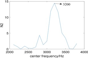
Fig. 2The curve of the relationship between N2 and bandwidth

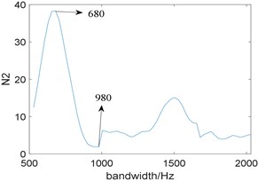
To explore the relationship between bandwidth and $N_2$, we fix the center frequency at 3200 Hz, and the bandwidth is selected between three times and eleven times of fault characteristic frequency, which is [555, 2035]. The corresponding curve of them is shown in Fig. 2, Where $N_2$ reaches the maximum when the bandwidth is 680 Hz, the minimum when the bandwidth is 980 Hz.

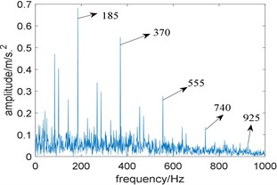
Fig. 3The squared envelope spectrum of the filtered signal at different bandwidth: a) the bandwidth 980 Hz, b) the bandwidth 680 Hz

a)

b)

In order to prove that $N_2$ is unreliable for selecting the bandwidth, two band-pass filters with a center frequency of 3200 Hz and bandwidths of 980 Hz and 680 Hz are designed respectively to filter the simulation signal and perform envelope demodulation. Fig. 3(a) is the squared envelope spectrum of the filtered signal at a bandwidth of 980 Hz, where fault characteristic frequency 185 Hz and its harmonics 370 Hz, 555 Hz and 740 Hz are clearly visible, and one of its harmonics 925 Hz can even been identified faintly. Fig. 3(b) is the squared envelope spectrum of the filtered signal when the bandwidth is 680 Hz, where only the fault characteristic frequency and two of its harmonics 370 Hz and 555 Hz can be identified. Comparing Fig. 3(a) with Fig. 3(b), the squared envelope spectrum of the filtered signal with the bandwidth of 980 Hz performs better. Therefore, $N_2$ is not appropriate for selecting the bandwidth.

From the above analyses, we come to the conclusion that $N_2$ is suitable for selecting the center frequency of the filter, but is unreliable for selecting the bandwidth. Hence, in this paper, the bandwidth is fixed at five times the fault characteristic frequency, and $N_2$ is utilized for selecting the optimal center frequency.

2.1.2. Whale optimization algorithm

Whale optimization algorithm [21] inspired by humpback whale hunting behavior is a meta-heuristic optimization algorithm, and its mathematical model can be expressed as the following three steps [21]:

1) Encircling prey.

Humpback whales can recognize the location of prey and encircle them, and this behavior can be represented by the following formulas:

8

$\left\{\begin{array}{l}D=\left|C{X}^{*}\left(t\right)-X\left(t\right)\right|,\\ X\left(t+1\right)=X^{*}\left(t\right)-AD,\end{array}\right.$

where $t$ indicates the current iteration, $X^{*}$ is the position vector of the best solution obtained so far, $X$ is the position vector, $\left|\bullet \right|$ is the absolute value, and ·stands for dot product. To obtain the optimal solution, the position of the whale needs to be updated according to the following formula during each iteration:

9

$\left\{\begin{array}{l}A=2ar-a,\\ C=2r,\end{array}\right.$

where $a$ linearly from 2 to 0 during the iterations and $r$ is selected randomly between 0 and 1.

2) Bubble-net attacking method.

The bubble-net attack method is a unique attack method for humpback whales. Two methods are designed to mathematically model its behavior.

The first method is shrinking encircling mechanism, which can be realized by reducing the value of $a$ in Eq. (9). The fluctuation range of $A$ is determined by the value of $a$. Here we set $A$ as random values in [–1, 1], then if $0\le A\le 1$, whales will attack towards the prey.

The second approach is called spiral updating position, which is utilized to mimic the helix-shaped movement of whales based on the position of the whale and prey. The formula can be represented as follows:

10

$X\left(t+1\right)=D\text{'}{e}^{bl}\mathrm{c}\mathrm{o}\mathrm{s}\left(2\pi l\right)+X\text{'}\left(t\right),$

where, $D\text{'}=\left|X^{*}\left(t\right)-X\left(t\right)\right|$ denotes the distance between the $i$th whale and its prey, $b$ is a constant utilized to simulate the shape of the logarithmic spiral, $l$ is selected randomly between –1 and 1.

To model the bubble-net attack method, assuming that the humpback whale has a 50 % probability of choosing a method to update its position, the following modeling can be performed:

11

$X\left(t+1\right)=\left\{\begin{array}{l}{X}^{*}\left(t\right)-AD,\begin{array}{ll}\mathrm{}\mathrm{}\mathrm{}\mathrm{}\mathrm{}\mathrm{}& 0\le p<0.5,\end{array}\\ D^{\text{'}}{e}^{bl}\mathrm{c}\mathrm{o}\mathrm{s}\left(2\pi l\right)+X^{*}\left(t\right),\begin{array}{ll}& \mathrm{}\mathrm{}0.5\le p\le 1,\end{array}\end{array}\right.$

where $p$ is a random number between 0 and 1.

3) Search for prey.

The same approach based on the variation of the $A$ vector can be utilized to search for prey, if $\left|A\right|\ge 1$, the search agent will be forced to move far away from a reference whale. This allows the WOA algorithm to perform a global search. The mathematical model is as follows:

12

$\left\{\begin{array}{l}D=\left|C{X}_{random}\left(t\right)-X\left(t\right)\right|,\\ X\left(t+1\right)=X_{random}\left(t\right)-AD,\end{array}\right.$

where, $X_{random}$indicates the random position vector selected from the current population.

According to the above analyses, The WOA algorithm can be illustrated as follows [15]:

Step 1: Initialize the whales’ population $X_i$($i=$1, 2,..., $n$).

Step 2: Initialize $a$, $A$, $C$, $l$ and $p.$

Step 3: Calculate the fitness of each search agent. $X^{*}$ is the best search agent;

Step 4: When $p<$0.5, if $\left|A\right|<$1, update the current population position with Eq. (8), else, update the current population position with Eq. (12); when 0.5 $<p<$1, use Eq. (10) to update the position of the current population;

Step 5: Update $a$, $A$ and $C$;

Step 6: Calculate the fitness of each search agent.

Step 7: Update the value of $X^{*}$.

Step 8: Determine whether the current iteration number $t<$ maximum number of iteration, if yes, repeat Steps 4 to 7. Else, return to $X^{*}$.

2.1.3. Using WOA to optimize filter center frequency

Considering the strong robustness of $N_2$ and the powerful optimization ability of WOA, this paper fixes the bandwidth at five times the fault characteristic frequency, then uses WOA to quickly select the optimal center frequency $X^{*}$, and $N_2$ is used as the objective function of WOA.

2.3. The principle of the proposed algorithm based on conditional variance statistic and cross-correlation spectrum

Considering that conditional variance statistic can be used as the objective function for selecting the center frequency of the filter, but not bandwidth, we choose to fix the bandwidth at five times the fault characteristic frequency, and use WOA to select the optimal center frequency quickly. To further suppress in-band noise, cross-correlation analysis based on higher order energy operator is utilized. In order to better display the proposed algorithm, the flowchart is shown in Fig. 4.

Fig. 4The flowchart of the proposed algorithm

3. Simulation verification

To verify the effectiveness of the proposed algorithm for extracting the fault feature, this section constructs a simulation signal under strong background noise, where repetitive transients and harmonic components are the same as those in for Eq. (7). The signal-to-noise ratio of the signal is –8.2 dB if no white noise is added, and the ratio is –15.2 dB after adding white noise.

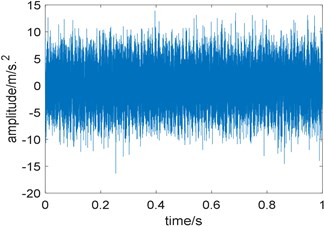
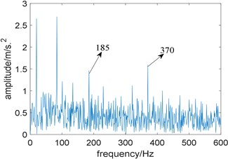
Fig. 5 are the time domain waveform of the simulation signal and its squared envelope spectrum. The envelope spectrum is obtained by performing Hilbert transform and FFT on the signal directly. Disturbed by strong background noise, repetitive transients related to the local damage can hardly be observed in the time domain waveform and only fault characteristic frequency 185 Hz along with one of its harmonics 370 Hz are able to be observed in the envelope spectrum.

Fig. 5Simulation signal: a) time domain waveform; b) squared envelope spectrum of a)

a)

b)

Fig. 6Time domain waveform of the filtered signal

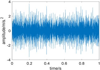
Fig. 7Results of the proposed method: a) the curve of FCI; b) cross-correlation spectrum

a)

b)

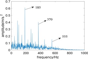
Next, the proposed algorithm is applied to the fault simulation signal. The fixed bandwidth is five times of fault characteristic frequency, namely 925 Hz; the optimal center frequency selected by whale optimization algorithm is 3270 Hz, which is basically consistent with the actual center frequency of 3200 Hz. Fig. 6 is the time domain waveform of the filtered signal, where background noise is significantly suppressed. Further, the filtered signal is analyzed by higher order energy operator. Fig. 7(a) shows the relationship between the order of energy operator and FCI, from which the optimal two energy operators with the largest FCI are selected for cross-correlation spectrum analysis, namely the fifth and ninth order; Fig. 7(b) is the cross-correlation spectrum, where noise components are obviously suppressed, fault characteristic frequency 185 Hz and its harmonics 370 Hz and 555 Hz are prominent, what’s more, the sidebands 101 Hz, 269 Hz, 412 Hz and 454 Hz which are modulated by rotating frequency can be observed too. Compared with Fig. 5(b), the proposed algorithm performs better.

In order to highlight the superiority of the proposed method, now we use Fast Kurtogram, EMD and Fast-SC [24] to deal with the simulation signal.

Fig. 8Results of fast kurtogram: a) the paving of fast kurtogram; b) the squared envelope spectrum of the signal filtered by fast kurtogram

a)

b)

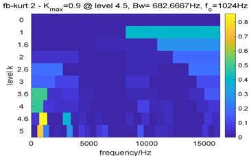
Fig. 8 are the results of Fast Kurtogram. Due to the interference of strong impulsive noise, the optimal center frequency determined by Fast Kurtogram is 1024 Hz, which is inconsistent with the actual center frequency, and the selected bandwidth is 682.7 Hz; the squared envelope spectrum of the selected frequency band showed in Fig. 8(b) also contains no useful information. Comparing Fig. 7(b) with Fig. 8(b), the proposed algorithm performs better.

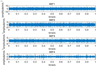
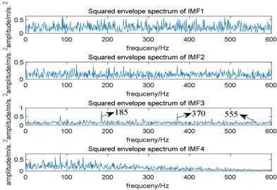
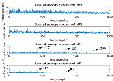
Since the useful components in the original signal are mostly concentrated in the first few intrinsic mode functions (IMF) obtained by EMD, we only take the first four IMFs for analysis. Fig. 9(a) is the time domain waveform of the first four IMFs and Fig. 9(b) is their squared envelope spectrum, from which we come to the conclusion that the third IMF contains the most useful information. To observe the performance of EMD more intuitively, we enlarge the squared envelope spectrum of the third IMF, which is shown in Fig. 10. In Fig. 10, although fault characteristic frequency 185 Hz and its harmonics can be observed, there still contains some noise interference. Comparing Fig. 7(b) with Fig. 10, the proposed algorithm performs better.

Fig. 9Results of EMD: a) the time domain waveform of the first four IMFs; b) the squared envelope spectrum of the first four IMFs

a)

b)

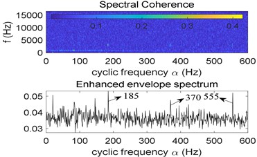
What is more, the analysis result of Fast-SC is shown in Fig. 11, where fault characteristic frequency and its harmonies can also be observed in its enhanced envelope spectrum. However, compared with Fig. 7(b), there still contains some noise interference, which indicates that the proposed algorithm performs better.

Fig. 10The squared envelope spectrum of the third IMF

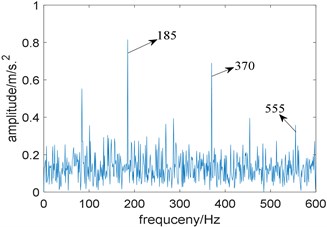
Fig. 11Result of Fast-SC

4. Experimental verification

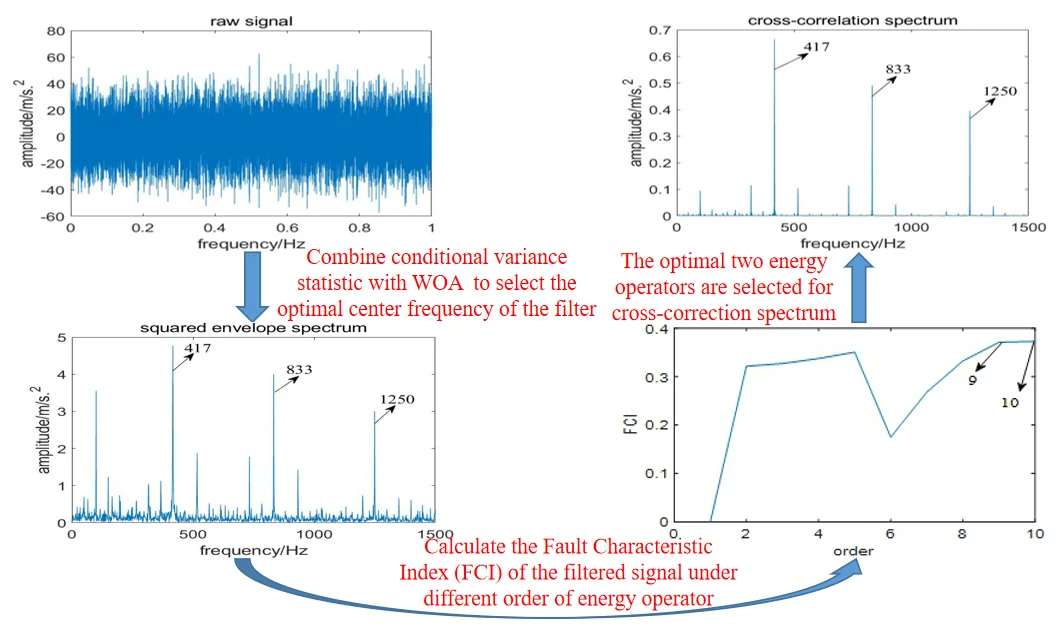
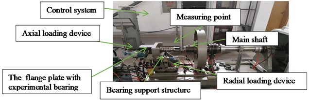
In this section, the vibration signal collected from a bearing test rig is analyzed to further evaluate the effectiveness of the proposed method for fault diagnosis of rolling element bearings. The test rig shown in Fig. 12 contains several main components, including bearing support structure, main shaft, experimental bearing, servo-driven motor, radial loading device, axial loading device and control system et al.

The experimental bearing type is 7010C with a local damage on the outer race generated by laser wire-electrode cutting, the fault size of the outer race was 0.5 mm (width) × 0.5 mm (depth). The outer diameter of the bearing is 80 mm and the inner diameter is 50 mm, the rolling element diameter is 8.7 mm, the number of rolling elements is 19, and the contact angle is 15°. The test speed is 3000 r/min, in order to obtain detailed signal data, the sampling frequency is set to the highest sampling frequency of the instrument, which is 131072 Hz, and the sampling time is 1 s. The theoretical fault characteristic frequency is calculated as 413.6 Hz.

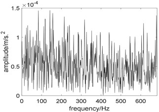
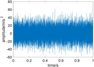
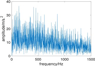
In order to reduce the calculation, the signal is resampled to 32768 Hz. Fig. 13 are the time domain waveform the experimental signal and its squared envelope spectrum. Due to the interference of strong background noise, repetitive transients related to local damage can hardly be observed in the time domain waveform and its squared envelope spectrum also contains no useful information.

Fig. 12The test rig

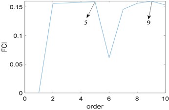
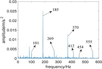
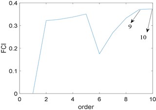
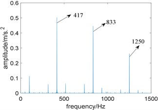
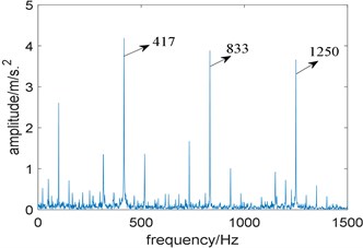
Next, the proposed algorithm is applied to the experimental signal. The bandwidth is fixed at five times fault characteristic frequency; the optimal center frequency selected by whale optimization algorithm is 2971 Hz. Fig. 14 is the time domain waveform of the filtered signal, compared with Fig. 13(a), noise interference is effectively suppressed. Further, the filtered signal is analyzed by higher order energy operator. Fig. 15(a) reflects the relationship between the order of energy operator and FCI, and the optimal two energy operators with the largest FCI are selected for cross-correlation spectrum analysis, namely the ninth and tenth order. Fig. 15(b) is the cross-correlation spectrum, it is obviously that noise components are suppressed, fault characteristic frequency 417 Hz and its harmonics 833 Hz and 1250 Hz are prominent. Compared with Fig. 13(b), the proposed algorithm performs better. What’s more, note that due to the fluctuation of the rotating speed or the sliding of the rolling bearing, the actual fault characteristic frequency is not equal to the theoretical value.

Fig. 13Experimental bearing vibration signal: a) time domain waveform; b) squared envelope spectrum of a)

a)

b)

Fig. 14Time domain waveform of the filtered signal

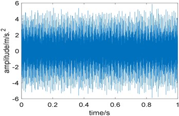
Fig. 15Results of the proposed method: a) the curve of FCI; b) cross-correlation spectrum

a)

b)

To further prove that $N_2$ is not suitable for selecting the bandwidth of the filter, we fix the center frequency at 2971 Hz, and the bandwidth is selected between three and eleven times of fault characteristic frequency. The relationship between $N_2$ and bandwidth is shown in Fig. 16, where $N_2$ reaches the maximum when the bandwidth is 2000 Hz, and the minimum when the bandwidth is 3100 Hz. Then two band-pass filters with a center frequency of 2971 Hz and bandwidths of 2000 Hz and 3100 Hz are designed to filter the experimental signal and perform envelope demodulation. Fig. 17(a) and Fig. 17(b) are the squared envelope spectrum of the filtered signal when the bandwidth is 2000 Hz and 3100 Hz, comparing Fig. 17(a) with Fig. 17(b), we find both of them perform well. Therefore, it is unreliable to select the bandwidth by $N_2$.

For comparison, Fast Kurtogram, EMD and Fast-SC are now utilized to analyze the experimental signal.

Fig. 16The curve of the relationship between N2 and bandwidth

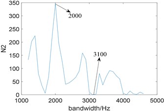
Fig. 17The squared envelope spectrum of the filtered signal at different bandwidth: a) the bandwidth 2000 Hz, b) the bandwidth 3100 Hz

a)

b)

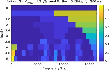
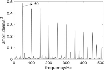
Fig. 18 are the results of Fast Kurtogram. Due to the interference of strong background noise, optimal center frequency determined by Fast Kurtogram is 256 Hz, and the selected bandwidth is 512 Hz; in the squared envelope spectrum of the optimal analysis frequency band, the prominent frequency 50 Hz corresponds to the rotation frequency of the rolling bearing, however, fault characteristic frequency and its harmonics cannot be Identified, which indicates Fast Kurtogram fails to extract the fault feature.

Fig. 18Results of fast kurtogram: a) the paving of fast kurtogram; b) the squared envelope spectrum of the signal filtered by fast kurtogram

a)

b)

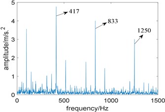
Similar to the simulation signal, we only give the time domain waveform and their squared envelope spectrum of the first four IMFs obtained by EMD, which is shown in Fig. 19, and the squared envelope spectrum of the third IMF which contains the most useful information is shown in Fig. 20. In Fig. 20, although fault characteristic frequency 417 Hz and its harmonics can be observed, there still exists some noise interference, compared with Fig. 15(b), the proposed algorithm performs better.

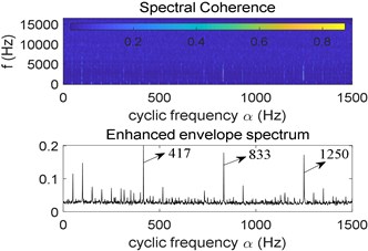
What’s more, the analysis result of Fast-SC is shown in Fig. 21, where fault characteristic frequency and its harmonies are also prominent. However, compared with Fig. 15(b), there still exists some noise interference in the enhanced envelope spectrum, so the proposed algorithm performs better.

Fig. 19Results of EMD: a) the time domain waveform of the first four IMFs; b) the squared envelope spectrum of the first four IMFs

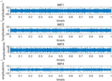
a)

b)

Fig. 20The squared envelope spectrum of the third IMF

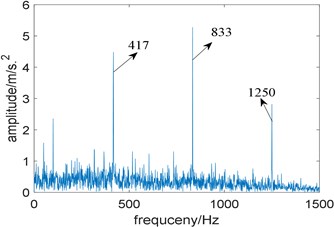
Fig. 21Result of Fast-SC

5. Conclusions

From the analyses of simulation and experimental signal, the algorithm proposed in this paper based on conditional variance statistic and cross-correlation spectrum analysis is feasible, and we have the conclusions as follow:

1) Compared with kurtosis and Gini index, conditional variance statistic is more robust and can be utilized as the objective function for selecting the optimal center frequency. However, we find that conditional variance statistic is undesirable for selecting the optimal bandwidth.

2) Finding the optimal center frequency by iteration will be affected by step size. If the step size is too long, the accurate center frequency cannot be selected; if the step size is too short, the calculation efficiency will be affected. In this paper, the bandwidth is fixed at five times fault characteristic frequency and WOA is applied to quickly select the optimal center frequency, what is more, $N_2$ is utilized as the objective function, so both of the calculation efficiency and accuracy of the selection of center frequency can be taken into consideration. To further suppress the noise interference, cross-correlation spectrum analysis is applied.

3) The analyses of the simulation and experimental signal indicate that the proposed method can effectively extract the fault feature of rolling bearings under strong background noise. Compared with classic Fast Kurtogram, EMD and Fast-SC, the proposed algorithm performs better.