Abstract
As essential equipment in rotating machinery, the fault diagnosis technology of rolling bearings has achieved great success. However, it still suffers from limitations in terms of generalization and noise resistance performance when operating under complex conditions. To accurately identify the fault types of rolling bearings under different loads and nosy environments, a novel intelligent fault diagnosis method is proposed. Firstly, the utilization of dilated convolution expands the network's receptive field, thereby effectively enhancing the scope of fault extraction. Then, by incorporating the Efficient Channel Attention (ECA) in different convolutional layers, the extracted features are adaptively recognized, highlighting important representation information and improving fault diagnosis performance. Finally, the proposed network is utilized for rolling bearing fault diagnosis under diverse operating and noise conditions, and its efficacy is evaluated on various datasets. The experimental results demonstrate that the proposed method exhibits good generalization performance and strong robustness, compared with other methods.
Highlights
- The dilated convolution expands the network's receptive field, effectively enhancing the scope of fault extraction.
- The ECA module intelligently focuses on significant features, thereby improving bearing fault diagnosis performance.
- The proposed model is validated using the CWRU and Qiqihar University bearing fault datasets. The experiments demonstrate its excellent generalization performance and strong robustness.
1. Introduction
Rolling bearings are widely applied in various modern mechanical equipment. However, under complex working conditions such as high speed, frequent load changes, rolling bearings are prone to occur aging and wear, which will lead to equipment damage, huge economic losses and even safety accidents. Therefore, to ensure normal and stable operation of mechanical equipment, fault diagnosis topic of rolling bearings has attracted more and more attention from engineers and experts [1, 2].
In recent years, two main methods for fault diagnosis have emerged: signal processing and intelligent diagnosis. The former includes technologies such as fast Fourier-transform (FFT) [3], empirical mode decomposition (EMD) [4], wavelet transform (WT) [5], variational mode decomposition (VMD) [6], and ensemble empirical pattern decomposition (EEMD) [7]. However, these methods are time-consuming and subjective due to the manual feature selection and limited professional knowledge of the experts. As a result, they may not provide satisfactory results under different working conditions. On the other hand, intelligent diagnosis technologies based on machine learning and deep learning have been widely used in various fields. In the field of fault diagnosis of rolling bearings, machine learning classification models such as artificial neural network (ANN) [8], support vector machine (SVM) [9], and principal component analysis (PCA) [10], have been successful in extracting correlation features from the original signal data to achieve an accurate diagnosis. Yan et al. [11] designed an improved SVM classification model to diagnose and classify rolling bearing faults by inputting information from different domains. Sharma et al. [12] proposed a bearing fault diagnosis method combining PCA and ANN. However, these models may not learn complex nonlinear relations from complex bearing vibration data. This is where deep learning technology comes in. With its deep network structure and unique advantages in signal processing and feature extraction [13], deep learning has been successfully applied in many fields, including fault diagnosis. Deep autoencoder (DAE), deep belief network (DBN), recurrent neural network (RNN), long short-term memory network (LSTM), and convolutional neural networks (CNN) are commonly used deep learning methods for fault identification. For example, Wang et al. [14] used the DBN model to extract fault features of planetary gear from raw signals and then used classifiers to identify fault types. Shao et al. [15] proposed an intelligent bearing fault diagnosis method that integrates deep autoencoders to overcome the difficulty of identifying the severity and direction of faults. The model overcomes the limitations of individual deep-learning models and achieves good diagnostic results. Mansouri et al. [16] used an improved RNN network to achieve excellent robustness in the fault detection and diagnosis of wind energy conversion systems (WEC). Gao et al. [17] proposed a diagnostic model that combines multi-channel continuous wavelet transform (MCCWT) with LSTM, which performs well under strong noise conditions. Chen et al. [18] proposed an intelligent diagnosis model that combines multi-scale convolutional neural networks and LSTM to identify bearing faults with high classification accuracy. Eren et al. [19] designed a compact and adaptive one-dimensional convolutional neural network to achieve real-time fault classification with an average accuracy of 93.2 % on the Case Western Reserve University dataset.
In the above literature, compared with other methods, the model based on deep learning has achieved better results in bearing fault diagnosis. However, in actual industrial production, deep learning techniques based on data-driven dealing with the data in variable load environments are usually prone to overfitting problems due to inconsistent data distribution, which leads to poor fault diagnosis performance. Therefore, to improve diagnostic performance, it is necessary to design a suitable deep network ensemble. Hao et al. [20] provided a method that combines a one-dimensional convolutional neural network and LSTM to achieve an effective diagnosis of bearings under variable operating conditions. Zhao et al. [21] proposed a normalized convolutional neural network with batch normalization and the exponential moving average technology, which had good stability for bearing fault diagnosis under different operating conditions. Zhang et al. [22] proposed a bearing fault diagnosis model applying a special training method that achieved an average accuracy of 95.5 % under different working loads. Peng et al. [23] designed a novel multibranch and multiscale convolutional neural network that can increase the depth of feature extraction and achieve good load domain adaptability on the bearing dataset. Jiao et al. [24] introduced an adversarial adaptation discriminator into the residual network, which was successfully applied to bearing fault detection. The above models have achieved fine results in multiple working conditions.
Due to the large data characteristic differences and noise interference in numerous operation conditions, it is difficult to obtain satisfactory results for fault diagnosis of rolling bearings. As a result, in order to improve the diagnosis ability in various working conditions and under different noise environments, a rolling bearing fault diagnosis method based on dilated convolution and efficient channel attention (ECA) is proposed. The proposed method exploits residual connections to improve the feature discriminative performance of the network. In addition, structure-stacked dilated convolutions with optimal dilated rate are inserted in the residual connection, which not only expands the receptive field of the network but also overcomes the grid effect for rolling bearing fault diagnosis. Moreover, the ECA module is introduced into the diagnosis network, which makes the extracted high weights adaptively assigned to important features, thereby further improving the fault diagnostic performance. Ultimately, the proposed method was tested on two bearing fault datasets in cross-load domains and different noise conditions. The results demonstrate that compared with the other methods, the proposed method has prominent performance in terms of generalization and anti-noise.
The rest of this paper is organized as follows. Section 2 introduces the theoretical fundamentals of dilated convolution, residual connection and the ECA module. Section 3 describes the proposed method in detail. Section 4 provides different contrast methods. Section 5 discusses the experimental results. Section 6 summarizes the whole paper and presents future work.
2. Background knowledge
2.1. Dilated convolution
Dilated convolution is first proposed to solve the problem of image resolution and information loss caused by down-sampling operations in image semantic segmentation tasks. Dilated convolution is a convolution method that can increase the receptive field of the original feature map, which can implement operations different from regular convolution. By setting different dilation rates, dilated convolution can ensure that the output feature size remains unchanged while more global feature information is extracted. The dilated convolution operation between the one-dimensional input and output can be expressed as follows:
where is the one-dimension signal input; represents convolution kernel; presents convolution operation; s is input feature length; and is the one-dimensional output. Normal convolution is a special case of dilated convolution. When = 1, the convolution layer is a traditional convolution layer. When the dilation rate is larger, the network obtains a larger receptive field than ordinary convolution. The calculation formula of ordinary convolution and dilated convolution kernel can be defined as follows:
where is the size of the normal convolution kernel; represents the dilation rate of the dilated convolution; represents the corresponding output under different dilation rates and convolution kernel sizes. For example, when the kernel size of the dilated convolution is 3 and the dilated rate is 2, it is equivalent to a normal convolution kernel size equal to 7. So it can effectively improve the feature extraction ability. However, due to multiple dilated convolution operations, there will be a lack of correlation between the associated information, and many features will not be fully extracted, resulting in the grid effect. Therefore, in this paper, in the stacking use of dilated convolutions, the dilation rates are set to= 1, 2, 3 for feature extraction. In this way, the grid effect can be avoided as much as possible, so as to deep features are effectively extracted and fault prediction and diagnosis are performed through classifiers in the fault diagnosis task.
2.2. Residual connection
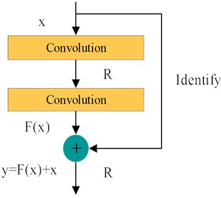
Experiments in the literature show that adding too many network layers to the deep model not only does not improve its training accuracy, but also leads to model degradation [25, 26]. To address this challenge, He proposed a residual structure with identity mapping in 2016 [27], and its structure is shown in Fig. 1. It can be seen from that the residual structure includes two convolutional layers, two ReLU activation functions and an identity shortcut connection. Moreover, the input and output vectors of the residual block are and , means the ReLU activation function. The output of the second convolutional layer can be expressed as , where and represent the weights of the two convolutional layers. The output of the residual block can be calculated as follows:
where (bias omitted for simplicity) is the residual mapping function. In the residual structure, the weight trained by the upper experiment layer is directly passed to rough the identity shortcut. when the network parameters are backpropagated, the use of the identity shortcut connection can effectively make the gradient flow to the upper layer close to , which is beneficial to update the parameters of the network. Such a design can avoid increasing network errors, which will cause the network to fall into local optimum or fail to converge.
Fig. 1Residual structure with the identify shortcut
2.3. ECA module
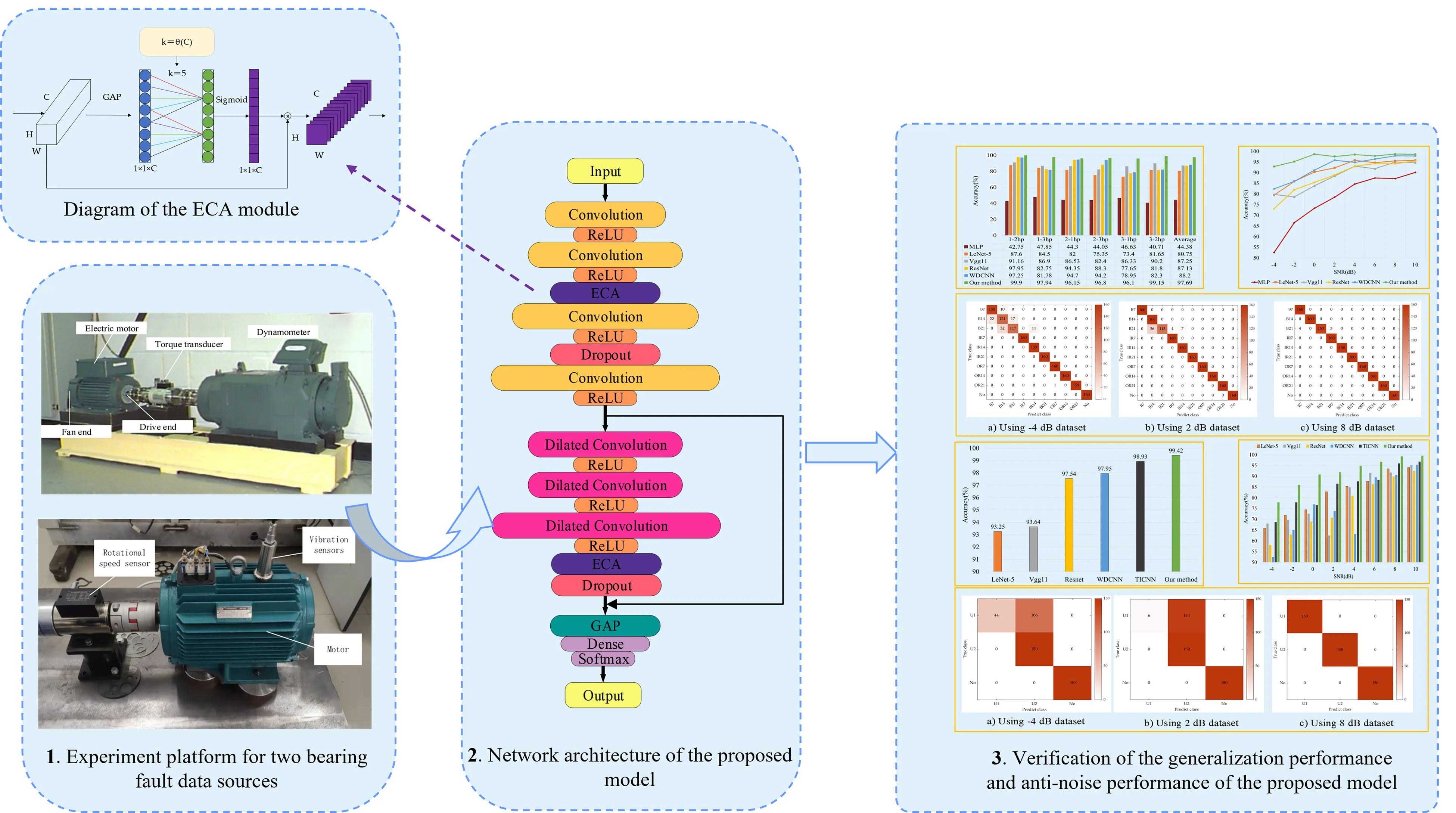
Different activation maps recognize fault features in different degrees, so some features may not be related to fault information or even indicate false information [28]. Therefore, this paper introduces the ECA module into the network, which serves as an attention mechanism for weight emphasis in the channel dimension, focusing on learning fault-related features [29]. It can improve the efficiency of extracting advanced features, which is beneficial to improve the performance of network models for fault diagnosis.
The basic structure of the ECA module is shown in Fig. 2. It can be seen that the focus feature is obtained by performing global average pooling (GAP) on each channel of the input feature map. Moreover, the convolution kernel size is adaptively obtained through Eq. (4), which generates the channel weights through the convolutional operation. Besides, the weight of each channel is calculated using the sigmoid nonlinear function. Finally, the weighted feature map is generated by multiplying the normalized weight and the original input feature map one by one. Eq. (4) is expressed as follows:
where represents the odd number closest to . The parameters and are are usually set to 2 and 1. The ECA module avoids the degradation of network performance caused by dimension reduction, and its limited parameters do not affect the computational complexity of the network.
3. Proposed method
3.1. Architecture of the network
In the actual production environment, rolling bearings often work in conditions with multiple load domains and noise interferences. Therefore, generalization performance and anti-noise ability are also significant indicators to evaluate network performance. Based on this, this paper proposes a novel fault diagnosis method for rolling bearings that combines one-dimensional dilated convolution with an attention mechanism. The network architecture is shown in Fig. 3. The raw signal collected from the vibration sensor is used as the network input. Next, the network structure mainly consists of one-dimensional convolution, dilated residual connection block, ECA module and global average pooling layer.
Fig. 2Diagram of the ECA module
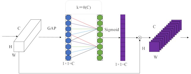
Fig. 3Architecture of the proposed network
First of all, the one-dimensional convolution layer can effectively extract and learn the original vibration information. Secondly, the dilated residual connection block can expand the receptive field of the network, thus improving the recognition accuracy of the network. Then, the ECA modules are embedded into the one-dimensional convolutional layer and the dilated residual connection block, which can adaptively calibrate important feature information and further improve network performance. In addition, the full-connected layer takes up a large number of parameters model and easily leads to overfitting of the network, so we use global average pooling instead of the full-connected layer to solve these problems. Finally, the fault diagnosis result is output through the softmax classifier of the full-connected layer.
3.2. Specific parameters of the network
The detailed parameters of the proposed method are summarized in Table 1. To ensure that the original signal samples input of the network contains enough periodic information, the input signal sample length is set to 2048×1. The network framework is mainly composed of one-dimensional convolution, the ECA module, and dilated convolution residual connection block. Specifically, one-dimensional convolution contains four layers with kernel sizes 16×1, 9×1, 6×1 and 3×1. Also, its number of channels is 16, 32, 64 and 128, respectively. Different kernel sizes could enable the network to learn feature information of different lengths. At the same time, the gradual increase in the number of channels can solve the problem of too many network parameters. Inspired by [27], we adopt stridden convolutions instead of max-pooling to focus feature information and reduce feature dimension without information loss. Therefore, the strides of the four convolutional layers are set to 1, 1, 2 and 4, respectively. In terms of the dilated convolutional residual connection block, it consists of 3 layers of dilated convolutions with different dilation rates and an ECA module. Then, the kernel size of the dilated convolutional layer is set to 3×1, and the number of kernel channels is set to 32, 32 and 128, respectively. Based on the consistency of the input and output feature dimension of the residual connection, the dilated convolution stride is set to 1, and the padding is set to “SAME”.
Table 1Detailed parameters of the network
No. | Type | Kernel | Channel | Stride | Output |
0 | Input | – | – | – | 2048×1 |
1 | Convolution layer 1 | 16×1 | 16 | 1 | 2048×16 |
2 | Convolution layer 2 | 9×1 | 32 | 2 | 1024×32 |
3 | ECA | - | – | – | 1024×32 |
4 | Convolution layer 3 | 6×1 | 64 | 2 | 512×64 |
5 | Convolution layer 4 | 3×1 | 128 | 4 | 128×128 |
6 | Dilated Convolution layer 1 | 3×1 | 32 | 1 | 128×64 |
7 | Dilated Convolution layer 2 | 3×1 | 32 | 1 | 128×64 |
8 | Dilated Convolution layer 3 | 3×1 | 128 | 1 | 128×128 |
9 | ECA | – | – | – | 128×128 |
10 | Global Average Pooling | – | – | – | 128 |
11 | Dense | – | – | – | 10 |
The proposed method is coded in Keras using TensorFlow backend and Python 3.8. Besides, it runs on a PC with NVIDIA GeForce GTX 940MX 2GB GPU under the WIN10 operating system. During the experiment, we use categorical cross-entropy as a loss function to evaluate the difference between the currently trained probability distribution and the real distribution. In addition, the Adam optimizer is used to optimize the loss function in the network. The batch size is chosen as 32. The experiment was repeated 5 times, and then the average value is selected as the final experimental result.
3.3. Contrast methods
In order to verify the validity of the proposed method for rolling bearing fault diagnosis, the contrast study with MLP, LeNet-5 [30], Vgg11 [31], Resnet, WDCNN [32], and TICNN [22] is performed in different datasets. It is noted that LeNet-5, Resnet and Vgg11, well-known deep learning networks, use two-dimensional (2D) grayscale images as input, which are obtained by matrix transformation from one-dimensional data. Furthermore, the other three methods directly take the original one-dimensional (1D) signals as inputs without any feature transformation. At present, there is no systematic approach to choose the most suitable hyper-parameters and structures of deep learning models [33]. Except the learning rate of MLP is 0.002, other models have been set to 0.001. In addition, the optimizer is set to Adam and the number of iterations is 30. Through numerous attempts in this study, the structures of MLP, Vgg11 and Resnet are determined empirically. The definite parameters of each model are set as follows:
MLP: the input of the model is the raw 1D vibration data. The model consists of three full-connected layers and one output layer. The number of neurons in the full-connected layer is 200, 200 and 50, respectively. The dropout operation is added after the first two full-connected layers.
LeNet-5: the model takes vibration data converted into 2D grayscale images as the input and contains two convolutional layers, two max-pooling layers and three full-connected layers. The first two convolutional layers contain 6 and 16 kernels respectively, and the size of the kernels is 5×5. The size and stride of the max-pooling kernel are both set as 2×2.
Vgg11: the model’s input is the 2D grayscale image consisting of 6 network blocks. The first 5 network blocks consist of a convolutional layer with a kernel size of 3×3 and a stride of 3×3, and each network block is followed by a max-pooling layer with a stride of 2×2. The sixth network block consists of three full-connected layers, with neurons 256, 256, and 10.
Resnet: the input is also the grayscale image converted from 1D data, consisting of one ordinary convolutional layer, three basic residual blocks, one global average pooling layer, and one full-connected layer. Batch normalization (BN) and max-pooling operation are respectively added after the convolutional layer. Furthermore, the number of channels in the three basic residual blocks is 64, 64 and 128, respectively among them, each basic residual block has two convolution layers with the same parameters, and the size of the convolution kernel is 3×3.
WDCNN: the model consists of five convolutional layers, five max-pooling layers and two full-connected layers. The activation function ReLU and BN operation are sequentially added between each convolutional layer and the maximum pooling layer. The kernel of the five convolutional layers is 16, 32, 64, 64 and 64 in sequence. The first convolutional layer has a larger kernel size. Moreover, the kernel size and stride of other convolutional layers are both set as 3×1 and 1×1. The kernel size and stride of all pooling operations are 2×1. The neural units in the two full-connected layers are 100 and 10.
4. Experimental results and analysis
4.1. Diagnosis results based on dataset A
To verify the fault diagnostic performance of the proposed method, dataset A obtained from the Bearing Data Center at Case Western Reserve University (CWRU) [34] was used in this study. The test rig of CWRU shown in Fig. 4 included primarily a 2 horsepower (hp) electric motor, a torque transducer, a dynamometer and control electrics. The Bearing vibration data at drive end and fan end were collected by the accelerometers using the 12 kHz sampling frequency. We chose the data at drive end to build dataset A performing in our network, as shown in Table 2. It can be seen that there are 10 kinds of bearing fault types in total, including normal, ball fault (from 0.007 to 0.021 inches), inner race fault (from 0.007 to 0.021 inches) and outer race fault (from 0.007 to 0.021 inches). According to the distribution differences of fault information under different working conditions, the dataset A is segmented into four different load domains sub dataset in turn, namely 0 hp, 1 hp, 2 hp and 3 hp. Samples of each fault class obtained through a fixed-step moving window are divided into training samples and testing samples at a ratio of 9:1.
To validate the generalization performance of the proposed method on different work conditions on Dataset A, Table 3 shows the prediction accuracy for bearing fault diagnosis under same loads testing, and Fig. 5 further compares the generalization ability of each method in the cross-load domains.
Fig. 4The test rig of CWRU
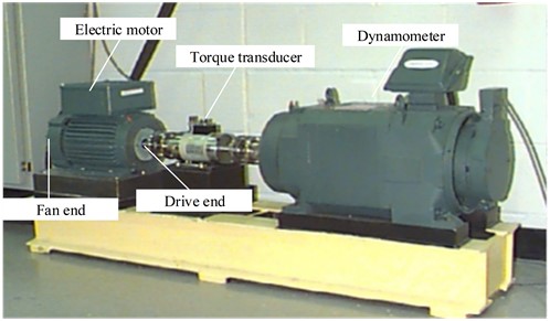
Table 2Description of dataset A
Fault condition | Diameter (inch) | Label | Load (hp) | |||
0 hp | 1 hp | 2 hp | 3 hp | |||
Ball | 0.007 | 0 | 400 | 400 | 400 | 400 |
Ball | 0.014 | 1 | 400 | 400 | 400 | 400 |
Ball | 0.021 | 2 | 400 | 400 | 400 | 400 |
Inner Race | 0.007 | 3 | 400 | 400 | 400 | 400 |
Inner Race | 0.014 | 4 | 400 | 400 | 400 | 400 |
Inner Race | 0.021 | 5 | 400 | 400 | 400 | 400 |
Outer Race | 0.007 | 6 | 400 | 400 | 400 | 400 |
Outer Race | 0.014 | 7 | 400 | 400 | 400 | 400 |
Outer Race | 0.021 | 8 | 400 | 400 | 400 | 400 |
Normal | 0 | 9 | 400 | 400 | 400 | 400 |
It is obvious from Table 3 that MLP performs poorly in learning fault characteristics, and the average accuracy is less than 93 %. In addition, the diagnosis accuracy of LeNet-5, Vgg11, and ResNet is 97.83 %, 92.51 % and 96.92 %, respectively. WDCNN shows higher accuracy than them. Our method has higher accuracy than WDCNN without attention mechanism. The accuracy of this method reaches 99.68 %, and the accuracy of WDCNN is 99.19 %. From the comparison results, the proposed method can effectively distinguish different fault types and fault severities under the same working conditions.
Table 3Diagnosis accuracy of different models under four loads
Methods | 0 hp | 1 hp | 2 hp | 3 hp | Average |
MLP | 86.98 | 90.93 | 94.79 | 95.43 | 92.01 |
LeNet-5 | 98.82 | 95.66 | 98.38 | 98.44 | 97.83 |
Vgg11 | 88.77 | 92.7 | 92 | 96.57 | 92.51 |
ResNet | 96.3 | 96.65 | 96.65 | 98.06 | 96.92 |
WDCNN | 99.43 | 97.56 | 99.93 | 99.83 | 99.19 |
Our method | 99.89 | 99.63 | 99.88 | 99.3 | 99.68 |
Rotating equipment inevitably operates under frequent load changes, so it is necessary to verify the stability of the proposed model under different Cross-load domains. Cross-load domains experiments are often used to evaluate the generalization ability of the model. The cross-load domains experiment means that one load domain data set is selected as the training set of the network model, and the others are used as testing data for classification prediction. For example, in this experiment, 1-2 hp and 1-3 hp represent that the network is trained at 1 hp, and 2 hp and 3 hp data are used for testing, respectively. The numerical results are presented in Fig. 5. It is obvious that the average diagnostic accuracy of our proposed method under cross-load domain conditions reaches 97.69 %, which is 53.31 %, 16.94 %, 10.44 %, 10.56 %, and 9.49 % higher than other comparative models, respectively. For cross-load domains experiments, the greater the degree of load variation, the higher the requirements for the generalization ability of the model. Taking 1-3 hp and 3-1 hp as examples, as a simple neural network, MLP based on machine learning is unable to perceive multiple range temporal feature representations and accurately predict fault characteristics, resulting in significantly lower diagnostic performance than other methods, with a diagnostic accuracy of only 47.85 % and 40.71 %.
Fig. 5Diagnosis accuracy of the cross-load domains
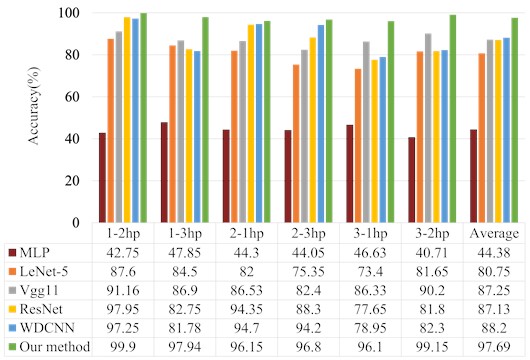
In addition, the higher diagnostic accuracy of LeNet-5, ResNet, and Vgg11 based on deep learning are 84.5 %, 86.9 %, and 81.78 %. This is because they use 2D data as the input, which will lead to the loss of the time domain characteristics of the original signal to a certain extent. Furthermore, the diagnostic accuracy of WDCNN in 1-3 hp and 3-1 hp group experiments only attains 81.78 % and 78.95 %, respectively, which are lower than Vgg11. The reason for such a result may be that WDCNN has too few layers so the advanced features contained in the signal cannot be fully extracted, resulting in a lower accuracy than Vgg11 with a higher network layer. The discriminant accuracy of our method in the case of 1-3 hp and 3-1 hp is higher than 97.94 % and 96.1 %, the highest is 97.94 %. This is because the range of features extracted by this method becomes wider due to adding the dilated convolutions. In addition, on account of the ECA module added, the extracted global knowledge is further distributed according to the weight, highlighting important features. Although the characteristics of training and test data are quite different in cross-load domains, this method can still effectively identify faults, showing its excellent generalization capacity.
To prove the excellent robustness of the proposed method, Gaussian white noise is added to the original dataset A to obtain composite data with different SNRs, thereby simulating various noisy environments. The diagnostic results are shown in Table 4 and Fig. 6. It is evident that our method compared to the others has a fine denoising capability in several noise environments, and the average diagnostic accuracy reaches 97.22 %. Furthermore, the identification accuracy of the MLP is the lowest among all models, only 77.54 %. This is because the features extracted by the MLP are short of the corresponding correlation, which affects the diagnostic performance. When the SNR of other methods is greater than 4 dB, the diagnostic accuracy exceeds 93 %, and the accuracy of the proposed method reaches the highest, which is 98.45 %. Although the diagnostic accuracy of the other methods also decreased rapidly while the SNR diminishes, the classification result of this network can still be more than 92.85 %. This is due to adding the dilated convolution in this model, which makes the features with noise deeply extracted, and the introduction of the attention mechanism makes it more sensitive to salient information. The diagnostic accuracy of WDCNN is 92.76 % only lower than this method. This is due to the large convolution kernel size of the first layer of the network, which has a certain filtering of noise information. Overall, the proposed method is more robust than the others for rolling bearing fault diagnosis.
Fig. 6Accuracy of different methods on dataset A
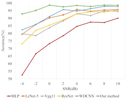
Table 4Anti-noise performance of different methods on dataset A
Methods | SNR (dB) | ||||||||
–4 | –2 | 0 | 2 | 4 | 6 | 8 | 10 | Average | |
MLP | 52.55 | 66.55 | 73.3 | 78.5 | 84.65 | 87.5 | 87.2 | 90.1 | 77.54 |
LeNet-5 | 79.45 | 85.9 | 90.3 | 92.25 | 95.75 | 94.65 | 95.5 | 95.75 | 91.19 |
Vgg11 | 79.79 | 78.62 | 83.83 | 88.43 | 93 | 91.83 | 94.97 | 94.66 | 88.14 |
ResNet | 73.1 | 81.95 | 85.45 | 88.9 | 93 | 94.25 | 94.15 | 95.5 | 88.29 |
WDCNN | 82.4 | 85.9 | 91.15 | 95.8 | 94.8 | 96.35 | 97.9 | 97.8 | 92.76 |
Our method | 92.85 | 95.15 | 98.65 | 97.55 | 98.45 | 97.8 | 98.7 | 98.6 | 97.22 |
Fig. 7Confusion matrix of the proposed method under different SNRs on dataset A
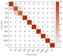
a) Using –4 dB dataset
b) Using 2 dB dataset
c) Using 8 dB dataset
To further evaluate the accuracy of the proposed model for bearing fault diagnosis, the classification results of four loads with different SNRs are summarized in the confusion matrix as shown in Fig. 7. The horizontal axis represents the number of predicted fault categories, and the vertical axis represents the number of true fault categories. The “B”, “IR”, “OR”, and “No” represents the fault types of ball fault, inner race fault, outer race fault and normal condition, respectively. The numbers following the abbreviation for failure types represent different fault diameters. For example, “B7” represents a ball fault with 0.007 inches. In the confusion matrix, it can be obviously seen that other faults compared to ball faults can be well distinguished when SNR is –4 dB. Specifically, the “B14” and “B12” types of faults are misjudged as other types of ball faults, and the numbers are 39 and 32, respectively. This may be due to the fact that different degrees of ball faults have similar characteristics in vibration sequences and vibration information is masked by strong noise, making it cannot effectively distinguish specific ball faults. When SNR increase from 2 dB to 8 dB, the number of misclassified ball faults decreases from 47 to 7, which means that the classification of ball faults is significantly improved due to the in-creased SNR.
4.2. Diagnosis results based on dataset B
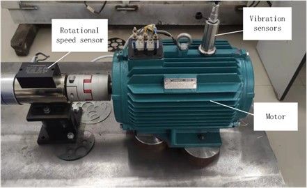
Dataset B was collected by the bearing fault experiment platform of Qiqihar University as shown in Fig. 8. It can be seen that the acceleration information is obtained through an acceleration sensor located above the special electric motor, and then the acceleration information was converted from the acquired analog signal to a digital signal in the microcontroller using an analog-to-digital converter. Furthermore, the sensor in two couplings was used to detect the motor rotation speed. The sampling frequency was set to 10 kHz, and each sequence of data lasted 10 seconds. In this experiment, the bearing fault data is only obtained under 2000 rpm. The dataset B considers three bearing health types, including normal, slight unbalanced fault and severe unbalanced fault. Each health type contains 1350 training samples, 150 validation samples and 150 testing samples.
Fig. 8Bearing experiment platform
To verify the diagnostic accuracy and anti-noise performance of the proposed method on dataset B, Fig. 9 shows the prediction accuracy of different methods, and Fig. 10 and Table 5 compare the anti-noise performance of different methods with SNR of –4 dB to 10 dB.
Table 5Anti-noise performance of different methods on dataset B
Methods | SNR (dB) | ||||||||
–4 | –2 | 0 | 2 | 4 | 6 | 8 | 10 | Average | |
MLP | 65.91 | 71.96 | 74.45 | 82.8 | 85.38 | 87.69 | 93.47 | 94.05 | 81.96 |
LeNet-5 | 68.06 | 69.6 | 72.61 | 62.46 | 84.89 | 91.59 | 91.7 | 95.2 | 79.51 |
Vgg11 | 58.04 | 62.93 | 68.93 | 70.76 | 80.89 | 86.4 | 89.91 | 92.44 | 76.29 |
ResNet | 52.49 | 65.07 | 76.98 | 73.91 | 63.24 | 89.51 | 90.62 | 95.33 | 75.89 |
WDCNN | 68.76 | 77.87 | 76.58 | 86.53 | 87.64 | 88.31 | 95.96 | 96.78 | 84.8 |
Our method | 77.91 | 86 | 90.8 | 91.87 | 94.84 | 96.71 | 99.24 | 99.6 | 92.12 |
It can be seen from Fig. 9 that the classification accuracy of the proposed method is higher compared with other methods. Table 5 and Fig. 10 reveal that the method has high anti-noise performance under different noise environments. As can be seen from Table 5, the adversarial noise capability of our method is significantly higher than the other methods in all SNR scenarios. Specifically, when the SNR is –4 dB, only the diagnostic accuracy of the proposed method is more than 70 %, which is 77.91 %. Although the classification performance of all methods improves significantly when the SNR is increased. Overall, the fault diagnosis performance of the proposed method is still better than other methods in different noise environments. The higher average diagnostic accuracy also demonstrates the noiseless advantage of the proposed method. It is worth noting that not every method improves the classification results while increasing the SNR. For example, when the SNR of the WDCNN is 2 dB and 4 dB, the diagnostic accuracy decreases. This may be due to the interference of the added signal on the original signal, which ultimately affects the network classification results.
Fig. 9Diagnosis results of different methods on dataset B
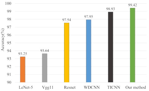
Fig. 10Accuracy of different methods on dataset B
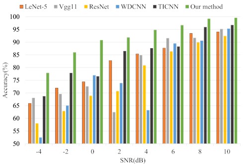
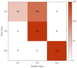
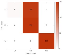
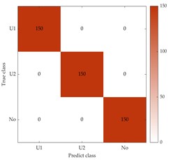
Fig. 11Confusion matrix of the proposed method under different SNRs on dataset B
a) Using –4 dB dataset
b) Using 2 dB dataset
c) Using 8 dB dataset
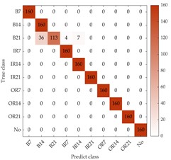
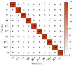
To better evaluate the diagnostic accuracy of the proposed method for different fault types on dataset B, the confusion matrix is calculated for –4, 2, and 8, as shown in Fig. 11. In Fig. 11, “U1” and “U2” represent slight and severe unbalanced faults, respectively, and “No” indicates normal, as in Fig. 7. The results shown in Fig. 11(a) indicate that only the mild unbalanced fault type was not well classified, with 144 samples misclassified as the severe unbalanced fault type. In Fig. 11(b, c), it should be noted that the number of misclassifications for slightly unbalanced fault types decreased from 106 to 0, indicating that all faults can be accurately distinguished while noise interference decreases.
5. Conclusions
The paper proposes a novel intelligent fault diagnosis method for rolling bearing that uses dilated convolution and attention mechanisms. The method incorporates residual connections and stacked dilated convolutions to improve the network’s feature extraction range and learning ability. An ECA module is embedded to focus on important features and promote the ability to extract fault information. The proposed method outperforms other methods in fault diagnosis performance under cross-load domains and diverse noise environments. The proposed method’s effectiveness is verified using two bearing fault datasets, showing good generalization performance and anti-noise ability. Currently, the work in this paper is only tested with a sufficient amount of data and has not been experimentally studied in real-time performance. In future research, we will further explore the fault diagnosis effect in the case of small samples, as well as real-time performance.
References
-
D. Gao, Y. Zhu, W. Kang, H. Fu, K. Yan, and Z. Ren, “Weak fault detection with a two-stage key frequency focusing model,” ISA Transactions, Vol. 125, pp. 384–399, Jun. 2022, https://doi.org/10.1016/j.isatra.2021.06.014
-
J. Jiao, M. Zhao, J. Lin, and C. Ding, “Deep coupled dense convolutional network with complementary data for intelligent fault diagnosis,” IEEE Transactions on Industrial Electronics, Vol. 66, No. 12, pp. 9858–9867, Dec. 2019, https://doi.org/10.1109/tie.2019.2902817
-
de Jesus Romero-Troncoso and Rene, “Multirate signal processing to improve FFT-based analysis for detecting faults in induction motors,” IEEE Transactions on Industrial Informatics, Vol. 13, No. 3, pp. 1291–1300, Jun. 2017, https://doi.org/10.1109/tii.2016.2603968
-
R. Valles-Novo, J. de Jesus Rangel-Magdaleno, J. M. Ramirez-Cortes, H. Peregrina-Barreto, and R. Morales-Caporal, “Empirical mode decomposition analysis for broken-bar detection on squirrel cage induction motors,” IEEE Transactions on Instrumentation and Measurement, Vol. 64, No. 5, pp. 1118–1128, May 2015, https://doi.org/10.1109/tim.2014.2373513
-
P. Sangeetha B. and H. S., “Rational-dilation wavelet transform based torque estimation from acoustic signals for fault diagnosis in a three-phase induction motor,” IEEE Transactions on Industrial Informatics, Vol. 15, No. 6, pp. 3492–3501, Jun. 2019, https://doi.org/10.1109/tii.2018.2874463
-
Y. Wang, Z. Wei, and J. Yang, “Feature trend extraction and adaptive density peaks search for intelligent fault diagnosis of machines,” IEEE Transactions on Industrial Informatics, Vol. 15, No. 1, pp. 105–115, Jan. 2019, https://doi.org/10.1109/tii.2018.2810226
-
Q. Fu, B. Jing, P. He, S. Si, and Y. Wang, “Fault feature selection and diagnosis of rolling bearings based on EEMD and optimized Elman_AdaBoost algorithm,” IEEE Sensors Journal, Vol. 18, No. 12, pp. 5024–5034, Jun. 2018, https://doi.org/10.1109/jsen.2018.2830109
-
B. Samanta, K. R. Al-Balushi, and S. A. Al-Araimi, “Artificial neural networks and genetic algorithm for bearing fault detection,” Soft Computing, Vol. 10, No. 3, pp. 264–271, Feb. 2006, https://doi.org/10.1007/s00500-005-0481-0
-
B. Samanta and C. Nataraj, “Use of particle swarm optimization for machinery fault detection,” Engineering Applications of Artificial Intelligence, Vol. 22, No. 2, pp. 308–316, Mar. 2009, https://doi.org/10.1016/j.engappai.2008.07.006
-
M. Misra, H. H. Yue, S. J. Qin, and C. Ling, “Multivariate process monitoring and fault diagnosis by multi-scale PCA,” Computers and Chemical Engineering, Vol. 26, No. 9, pp. 1281–1293, Sep. 2002, https://doi.org/10.1016/s0098-1354(02)00093-5
-
X. Yan and M. Jia, “A novel optimized SVM classification algorithm with multi-domain feature and its application to fault diagnosis of rolling bearing,” Neurocomputing, Vol. 313, pp. 47–64, Nov. 2018, https://doi.org/10.1016/j.neucom.2018.05.002
-
A. Sharma, L. Mathew, S. Chatterji, and D. Goyal, “Artificial intelligence-based fault diagnosis for condition monitoring of electric motors,” International Journal of Pattern Recognition and Artificial Intelligence, Vol. 34, No. 13, p. 2059043, Dec. 2020, https://doi.org/10.1142/s0218001420590430
-
G. E. Hinton and R. R. Salakhutdinov, “Reducing the dimensionality of data with neural networks,” Science, Vol. 313, No. 5786, pp. 504–507, Jul. 2006, https://doi.org/10.1126/science.1127647
-
X. Wang, Y. Qin, and A. Zhang, “An intelligent fault diagnosis approach for planetary gearboxes based on deep belief networks and uniformed features,” Journal of Intelligent and Fuzzy Systems, Vol. 34, No. 6, pp. 3619–3634, Jun. 2018, https://doi.org/10.3233/jifs-169538
-
H. Shao, H. Jiang, Y. Lin, and X. Li, “A novel method for intelligent fault diagnosis of rolling bearings using ensemble deep auto-encoders,” Mechanical Systems and Signal Processing, Vol. 102, pp. 278–297, Mar. 2018, https://doi.org/10.1016/j.ymssp.2017.09.026
-
M. Mansouri, K. Dhibi, M. Hajji, K. Bouzara, H. Nounou, and M. Nounou, “Interval-valued reduced RNN for fault detection and diagnosis for wind energy conversion systems,” IEEE Sensors Journal, Vol. 22, No. 13, pp. 13581–13588, Jul. 2022, https://doi.org/10.1109/jsen.2022.3175866
-
D. Gao, Y. Zhu, Z. Ren, K. Yan, and W. Kang, “A novel weak fault diagnosis method for rolling bearings based on LSTM considering quasi-periodicity,” Knowledge-Based Systems, Vol. 231, p. 107413, Nov. 2021, https://doi.org/10.1016/j.knosys.2021.107413
-
X. Chen, B. Zhang, and D. Gao, “Bearing fault diagnosis base on multi-scale CNN and LSTM model,” Journal of Intelligent Manufacturing, Vol. 32, No. 4, pp. 971–987, Apr. 2021, https://doi.org/10.1007/s10845-020-01600-2
-
L. Eren, T. Ince, and S. Kiranyaz, “A generic intelligent bearing fault diagnosis system using compact adaptive 1D CNN classifier,” Journal of Signal Processing Systems, Vol. 91, No. 2, pp. 179–189, Feb. 2019, https://doi.org/10.1007/s11265-018-1378-3
-
S. Hao, F.-X. Ge, Y. Li, and J. Jiang, “Multisensor bearing fault diagnosis based on one-dimensional convolutional long short-term memory networks,” Measurement, Vol. 159, p. 107802, Jul. 2020, https://doi.org/10.1016/j.measurement.2020.107802
-
B. Zhao, X. Zhang, H. Li, and Z. Yang, “Intelligent fault diagnosis of rolling bearings based on normalized CNN considering data imbalance and variable working conditions,” Knowledge-Based Systems, Vol. 199, p. 105971, Jul. 2020, https://doi.org/10.1016/j.knosys.2020.105971
-
W. Zhang, C. Li, G. Peng, Y. Chen, and Z. Zhang, “A deep convolutional neural network with new training methods for bearing fault diagnosis under noisy environment and different working load,” Mechanical Systems and Signal Processing, Vol. 100, pp. 439–453, Feb. 2018, https://doi.org/10.1016/j.ymssp.2017.06.022
-
D. Peng, H. Wang, Z. Liu, W. Zhang, M. J. Zuo, and J. Chen, “Multibranch and multiscale CNN for fault diagnosis of wheelset bearings under strong noise and variable load condition,” IEEE Transactions on Industrial Informatics, Vol. 16, No. 7, pp. 4949–4960, Jul. 2020, https://doi.org/10.1109/tii.2020.2967557
-
J. Jiao, M. Zhao, J. Lin, and K. Liang, “Residual joint adaptation adversarial network for intelligent transfer fault diagnosis,” Mechanical Systems and Signal Processing, Vol. 145, p. 106962, Nov. 2020, https://doi.org/10.1016/j.ymssp.2020.106962
-
K. He and J. Sun, “Convolutional neural networks at constrained time cost,” in IEEE Computer Society Conference on Computer Vision and Pattern Recognition (CVPR), pp. 5353–5360, 2014, https://doi.org/10.48550/arxiv.1412.1710
-
R. K. Srivastava, K. Greff, and J. Schmidhuber, “Highway networks,” arXiv:1505.00387, 2015.
-
K. He, X. Zhang, S. Ren, and J. Sun, “Deep residual learning for image recognition,” in 2016 IEEE Conference on Computer Vision and Pattern Recognition (CVPR), pp. 770–778, Jun. 2016, https://doi.org/10.1109/cvpr.2016.90
-
H. Wang, Z. Liu, D. Peng, and Y. Qin, “Understanding and learning discriminant features based on multiattention 1DCNN for wheelset bearing fault diagnosis,” IEEE Transactions on Industrial Informatics, Vol. 16, No. 9, pp. 5735–5745, Sep. 2020, https://doi.org/10.1109/tii.2019.2955540
-
Q. Wang, B. Wu, P. Zhu, P. Li, W. Zuo, and Q. Hu, “ECA-Net: Efficient channel attention for deep convolutional neural networks,” in 2020 IEEE/CVF Conference on Computer Vision and Pattern Recognition (CVPR), pp. 14–19, Jun. 2020, https://doi.org/10.1109/cvpr42600.2020.01155
-
Y. Lecun, L. Bottou, Y. Bengio, and P. Haffner, “Gradient-based learning applied to document recognition,” Proceedings of the IEEE, Vol. 86, No. 11, pp. 2278–2324, 1998, https://doi.org/10.1109/5.726791
-
K. Simonyan and A. Zisserman, “Very deep convolutional networks for large-scale image recognition,” in International Conference on Learning Representations (ICLR), pp. 7–9, 2014, https://doi.org/10.48550/arxiv.1409.1556
-
W. Zhang, G. Peng, C. Li, Y. Chen, and Z. Zhang, “A new deep learning model for fault diagnosis with good anti-noise and domain adaptation ability on raw vibration signals,” Sensors, Vol. 17, No. 2, p. 425, Feb. 2017, https://doi.org/10.3390/s17020425
-
S. Xing, Y. Lei, S. Wang, and F. Jia, “Distribution-invariant deep belief network for intelligent fault diagnosis of machines under new working conditions,” IEEE Transactions on Industrial Electronics, Vol. 68, No. 3, pp. 2617–2625, Mar. 2021, https://doi.org/10.1109/tie.2020.2972461
-
T. Matsubara and H. Torikai, “An asynchronous recurrent network of cellular automaton-based neurons and its reproduction of spiking neural network activities,” IEEE Transactions on Neural Networks and Learning Systems, Vol. 27, No. 4, pp. 836–852, Apr. 2016, https://doi.org/10.1109/tnnls.2015.2425893
About this article

This research is supported by the joint guiding project of the Natural Science Foundation of Heilongjiang Province (approved grant: LH2019F038), the Scientific Research Foundation of the Education Department of Heilongjiang Province (approved grant: 145209409) and the project of the Postgraduate Innovative Research of the Qiqihar University (approved grant: YJSCX2022046).
The datasets generated during and/or analyzed during the current study are available from the corresponding author on reasonable request.
Hui Zhang: supervision. Shengdong Liu: writing -original draft preparation. Ziwei Lv: Validation. Zhenlong Sang: software. Fangning Li: visualization.
The authors declare that they have no conflict of interest.
