Abstract
Vibration signal produced by rolling element bearings has obvious non-stationary and nonlinear characteristics, and it’s necessary to preprocess the original signals to obtain better diagnostic results. This paper proposes an improved variational mode decomposition (IVMD) and deep convolutional neural network (DCNN) method to realize the intelligent fault diagnosis of rolling element bearings. Firstly, to solve the problem that the number of decomposed modes of variational mode decomposition (VMD) needs to be preset, an IVMD method is proposed, where the mode number can be determined adaptively according to the curve of the instantaneous frequency mean of mode functions. With this method, the vibration signal can be decomposed into a series of modal components containing bearing fault characteristic information. Then, DCNN is employed to fuse these multi-scale modal components, which can automatically learn fault features and establish bearing fault diagnosis model to realize intelligent fault diagnosis eventually. Experimental analysis and comparison results verify that the proposed method can effectively enhance the bearing fault features and improve the diagnosis accuracy.
Highlights
- This paper proposed a signal processing method based on improved VMD method.
- The mode number of VMD can be determined adaptively according to the curve of the instantaneous frequency mean of mode functions.
- DCNN is employed to establish bearing fault diagnosis model to realize intelligent fault diagnosis.
1. Introduction
Rolling element bearings are the most critical parts in the rotating machinery. So accurate and reliable fault diagnosis of rolling element bearing is of great significance to maintain normal operation of mechanical equipment [1, 2].
The vibration signal of rolling element bearing contains a large amount of operating status information. Extracting sensitive and effective fault features is the key to bearing fault diagnosis [3]. When a rolling element bearing fails, its vibration signal appears as a distinct non-stationary and multi-component modulated signal because of the influence of its structure, operation mode, transmission path and load fluctuation [4], which is easy to be interfered by external noise. Therefore, it is necessary to pre-process the vibration signal of rolling element bearing to obtain better diagnostic results. Several adaptive non-stationary signal analysis methods have been proposed over the years, such as local mean decomposition (LMD), Empirical mode decomposition (EMD) and ensemble empirical mode decomposition (EEMD). LMD can adaptively decompose a complex multi-component signal into several product functions and a residual component, and has good nonlinear and non-stationary signal analysis capabilities [5]. EMD is a time-frequency signal processing method proposed by Huang [6], which can adaptively decompose complex nonlinear and non-stationary signals into a series of intrinsic mode function (IMF) [7]. However, EMD may produce modal aliasing and boundary effect in the decomposition process. EEMD was proposed by Wu and Huang [8], and applied in bearing fault feature extraction [9], which added white noise to the analyzed signal. Although EEMD improves the aliasing problem of EMD, it is still a recursive filtering algorithm like EMD. Aiming at this problem, Dragomireteskiy [10] proposed a completely non-recursive adaptive signal decomposition method-variational mode decomposition (VMD), which is decomposed by solving a constrained variational problem. VMD converts mode decomposition into non-recursive and variable decomposition problems, avoiding the problems of mode aliasing and boundary effect caused by recursive decomposition. Moreover, VMD has solid mathematical theory and better noise robustness. However, VMD has an obvious disadvantage that it needs to set the mode number of decompositions in advance. If the preset number of decompositions is not accurate, it may result in significant modal loss or mixed signal components. At present, the mode number of VMD is mainly determined by the central frequency observation method, which requires a given number of modes in advance and relies on manual experience. Obviously, it limits the adaptability of VMD in practical application. For this reason, Jiang [11] proposed a coarse-to-fine decomposing strategy, where the initial balance parameter is given roughly and the optimal target mode is determined by adjusting the balance parameter finely. Li [12] proposed a parametric adaptive VMD method to reduce the influence of artificially setting decomposition number, and applied it to the fault diagnosis of planetary gear box. To solve this problem, this paper proposes an IVMD method to select the appropriate mode decomposition number according to the change of instantaneous frequency mean of modal component.
In recent years, some scholars have combined VMD with fault feature extraction and pattern recognition for bearing fault diagnosis and achieved good results. For example, Jiang [13] combined VMD with fuzzy C-means clustering to identify rolling element bearing faults. These methods all adopt the common pattern recognition algorithm based on “shallow learning”. After signal decomposition, manual design and feature extraction are still needed. Meanwhile, the model has a limit on expression ability of complex functions and poor generalization ability.
As a typical representative of the new generation of artificial intelligence technology, deep learning has been successfully applied in the fields of speech recognition and image processing [14, 15]. Convolutional neural network (CNN) is one of the most widely used deep learning models. It achieves local connection through convolutional operation to reduce the complexity of the network and reduces the computational complexity through weight sharing in the learning process. For these reasons, CNN has also been applied in machinery fault diagnosis [16, 17]. For example, Jia [17] proposed a deep normalized convolutional neural network to solve the problem of imbalanced fault classification of machinery and applied it to bearing fault diagnosis. These studies show that CNN can reduce the uncertainty caused by artificial feature design and extraction in fault diagnosis and the dependence on expert diagnostic knowledge. Deep CNN (DCNN) is constructed by deepening the CNN network depth, which can obtain the complex mapping relationship between equipment monitoring data and running state through layer-by-layer abstract learning. In view of this trait, it is very suitable for the mechanical intelligent fault diagnosis under the background of complex data.
In this paper, a novel fault diagnosis method for rolling element bearings is proposed. Firstly, IVMD is adopted to preprocess the rolling element bearing signals. And then several modal components containing obvious fault information are taken as the input of DCNN model. Finally, DCNN is used to realize intelligent fault diagnosis of rolling element bearing. The remainder of this paper is composed as follows. Section 2 explains the theory of VMD briefly and proposes an IVMD method. In Section 3, the structure of DCNN is introduced. In Section 4, the proposed diagnosis method based on IVMD and DCNN is described. In Section 5, experimental verification of the proposed method is conducted. IVMD is combined with DCNN to analyze rolling element bearing signals of ten different states. Finally, conclusions are given in Section 6.
2. IVMD
2.1. Variation mode decomposition theory
VMD can divide the frequency domain signal adaptively and separate each component effectively. Assuming that VMD decomposes the original input signal into mode functions, steps for constructing the variational problem are as follows:
Step 1: Perform Hilbert transformation on sub-signals (modes) to calculate the unilateral frequency spectrum of analytic signal as shown in Eq. (1):
where is the impulse function, is mode ensemble, and is the mode number.
Step 2: is multiplied by the analytic signal of each , and modulating the frequency spectrum of each modal component to the corresponding fundamental frequency band, modal function is as follows:
Step 3: By calculating the squared norm of each demodulation signal gradient after translation and estimating the bandwidth of each mode function, the mathematical description of the final constrained variational problem is shown as follows:
where is the partial derivative of the function, is center frequencies of .
In order to solve the constrained variational problem, the Lagrangian multiplier and the quadratic penalty term are introduced to render the problem into an unconstrained variational problem. The extended Lagrangian expression is shown as follows:
Aiming at the problem Eq. (4), VMD uses the alternate direction method of multipliers (ADMM) to get the optimal solution of the constrained variational model.
At first, the decomposition number of the modal needs to be set in advance, and , , should be initialized. Then, according to Eqs. (5) and (6), the mode function and their central frequency are updated alternately:
The Lagrangian multiplier is also updated according to the following Eq. (7):
Repeat the above updating iteration until the convergence condition Eqs. (8) is satisfied:
2.2. Improved variational mode decomposition
In VMD, the decomposition number needs to be preset artificially. When is too small, decomposition will cause the loss of some crucial information. When is too large, the calculation amount of VMD is increased, and frequency aliasing is easy to occur. Therefore, selecting suitable number of decomposition modes is vital in VMD.
This paper proposes a method to determine the number of based on the change of instantaneous frequency mean of modal component. Instantaneous Frequency (IF) is the derivative of the phase of complex analytic signal, which is an important physical quantity to describe the characteristics of nonstationary signals. IF is based on the Hilbert transform and has instantaneous validity. Assuming that the original signal is decomposed by VMD to obtain modal components, each of mode has points, the expression of mean of IF is established as follows:
where denotes the th point of the th mode component, is the number of instantaneous frequencies obtained by instfreq function after Hilbert transformation of the th mode component.
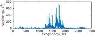
For illustrating and verifying the method, the outer ring fault model is used to simulate the periodic impact signal generated by bearing fault, and white noise is added into it. The expression of simulation signal is constructed as follows:
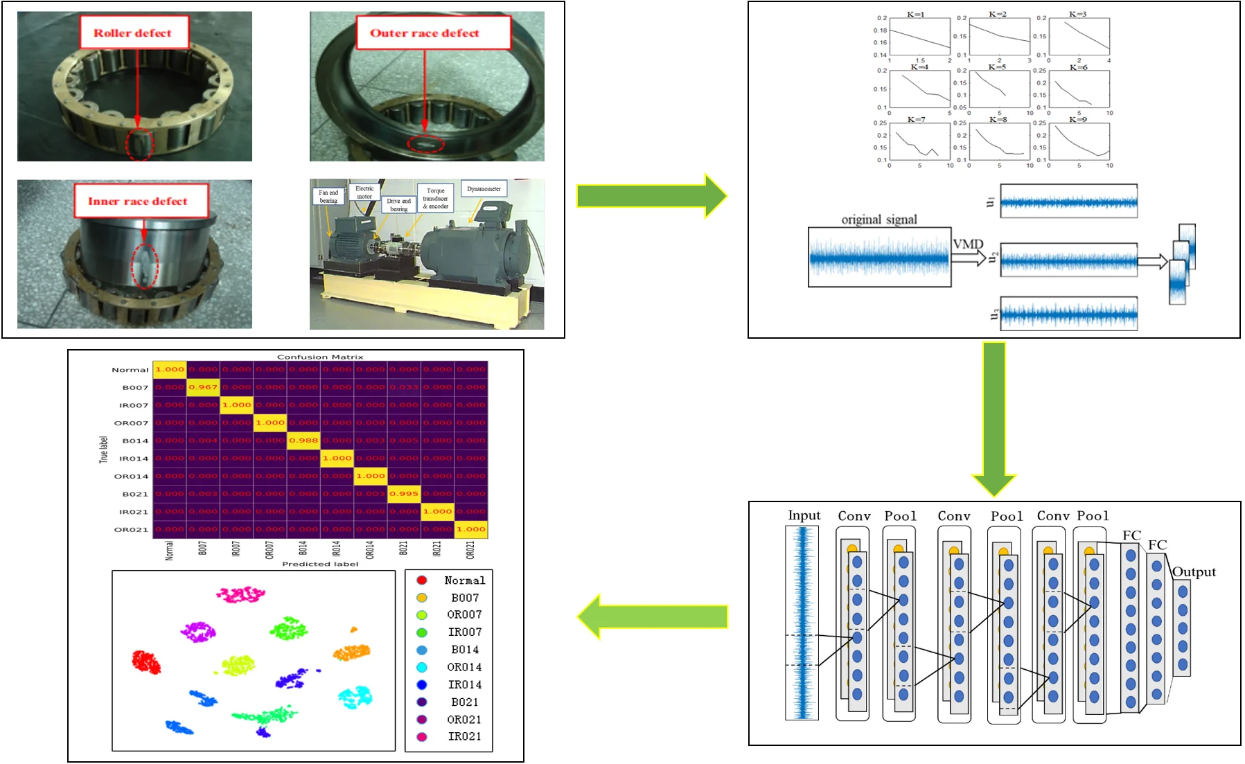
In the above equation, the carrier frequency is 3000 Hz, the displacement of constant 3, the Damping coefficient is 0.05, the period of impact failure is 0.01 s, the sampling frequency is 12 kHz, the sampling points is 4096, the sampling time is , and the white noise is . The simulated time domain waveform is shown in Fig. 1.
Fig. 1Simulated vibration signal of rolling bearing with outer race fault
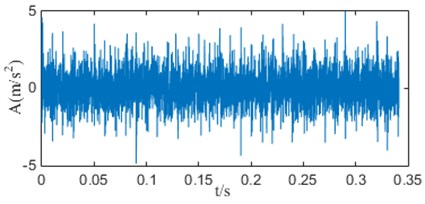
On the premise that the quadratic penalty term is constant, when is 1 to 9, the IF mean curves of the simulation signal decomposed by VMD is shown in Fig. 2.
When , the curves all appear an obvious downward bending. It can be explained that when is too large, frequency aliasing will occur in the modal components and intermittent phenomenon will appear. Especially in the high frequency, it causes the mean of IF to drop suddenly, which is the root of the curve bending phenomenon. When is less than 4, the curve is approximately a straight line, indicating that there is no mode mixing phenomenon in the decomposed components. However, when is too small, VMD algorithm will filter out some important information in the original signal. Therefore, the number of decomposed modes is determined to be the critical 3 before the curve is bending down.
Fig. 2Instantaneous frequency mean curves of modal components under different K values
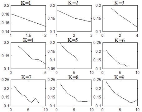
In order to automatically judge the bending down of the curve, second derivative is calculated and adopted as a numerical criterion. If signs of second derivative at two adjacent points are opposite and their absolute difference is greater than 0.05, an obvious bending down phenomenon can be found in the curve. It should be noted that 0.05 is a threshold obtained by many trials, which can avoid subtle fluctuations in the curve. To explain this criterion, the instantaneous frequency mean curve of 4 in Fig. 2 is taken as an example and shown in Fig. 3.
Fig. 3The instantaneous frequency mean curves of K= 4
In Fig. 3, A, B, C and D are the points of the instantaneous frequency mean of the modal components , , and . The value of second derivative and the second derivative can be calculated as 0.023 and –0.032. and are opposite signs and their absolute difference is greater than 0.05. Therefore, according to the change of curvature, 4 is the inflection point where the curve has been bending down. So, a suitable decomposition number can be determined to be 3.
3. Deep convolutional neural network
DCNN is a feedforward neural network, whose structure is shown in Fig. 4, including input layer, convolution layer, pooling layer, full connection layer and output layer. The convolutional layer contains multiple feature maps, and each is composed of multiple neurons. Each neuron is locally connected to the feature map of the previous layer through the convolution kernel. The operation of convolution layer is to extract features [18]. After the convolution operation, it is necessary to use the activation function to increase its nonlinear transformation ability. In this model, Rectified Linear Unit (ReLU) function is adopted as the activation function.
Fig. 4The structure of DCNN
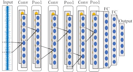
Pooling layer generally has two functions. One is to reduce the dimension of features while extracting significant features. The second is to control over-fitting and improve the performance of the model. Common pooling methods include average pooling, maximum pooling and random pooling. The maximum pooling is selected in this model.
Fully connected (FC) layer acts as a “classifier” in the whole CNN. All local features extracted by multiple alternating convolutional layers and pooling layers are summarized to the fully connected layer. Finally, the bearing fault classification is realized by softmax classifier.
4. Bearing fault diagnosis based on IVMD and DCNN
4.1. Processing of original vibration data
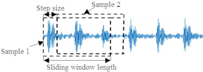
Since DCNN fault diagnosis model requires more samples for training, sliding window shown in Fig. 5 is adopted to intercept the original vibration data to construct samples.
Fig. 5Sample construction with sliding window
4.2. Diagnostic process
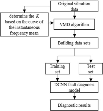
The flow of rolling element bearing fault diagnosis method based on IVMD and DCNN is shown in Fig. 6, and specific steps are shown as follows:
Steps 1: Process the original vibration data of rolling element bearings by sliding window, and the vibration data samples in different states are obtained.
Steps 2: The number of modes is determined according to the IF mean curve. Then, use VMD to decompose vibration data into modal components.
Steps 3: Stack all the decomposed components into a multi-channel sample in order. Then the whole dataset is divided into training set and test set.
Steps 4: Train the designed DCNN model with training dataset. Finally, diagnosis results can be obtained by inputting the test data into the trained DCNN model.
Fig. 6Flow of bearing fault diagnosis method based on IVMD and DCNN
5. Experiment
5.1. Description of experimental data
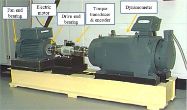
In order to verify the effectiveness and feasibility of the proposed method, the rolling element bearing experimental data provided by Bearing Data Center of Case Western Reserve University (CWRU) [19] is used in this study. The basic layout of the test rig is shown in Fig. 7, it consists of a 2 HP motor, a torque sensor, dynamometer and control electronics. The vibration data with inner race, rolling ball and outer race fault were collected at the drive end bearing. The sampling frequency of the experiment data is 12 kHz, and the rotating speed of shaft is 1727 r/min, namely the rotating frequency is 28.78 Hz.
Bearing state is divided into four types: normal, inner ring fault, outer ring fault and rolling element fault. The defect sizes are 0.007 in, 0.014 in, and 0.021 in respectively, and ten different rolling element bearing states are obtained. The sliding window is adopted to segment the original vibration data. The sliding length is set as 1200, and the moving step length is set as 50. Eventually, there are 1500 samples in each state, and each sample contains 1200 data points.
Fig. 7Test rig of CWRU
5.2. Data preprocessing based on IVMD algorithm
Firstly, IVMD is used to process rolling bearing signals in ten states. For brevity, Fig. 8 shows the decomposition results of four health conditions with fault defects of 0.14 in, including normal condition, inner race fault, outer race fault and rolling element fault conditions. It can be seen that when 4, all the instantaneous frequency curves show obvious downward bending. Similar phenomenon can also be observed in other states. Then, according to the change of curvature, the downward bending point of the bearing signal in ten states is judged to be at 4.
Fig. 8Instantaneous frequency mean curves of modal components under different K
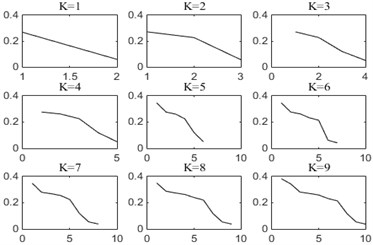
a) Normal
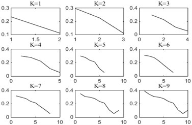
b) IR014
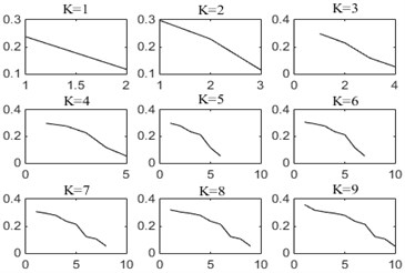
c) OR014
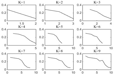
d) B014
In order to further explain the cause of the curve bending down, the signal of inner ring fault is decomposed by the VMD under different number of modes , and the spectrums of original signal and each mode component are shown in the Fig. 9.
Fig. 9The original signal and spectrum of various modal components at different K values
a) The spectrum of original signal
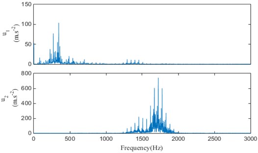
b) Spectrums of mode components when 2
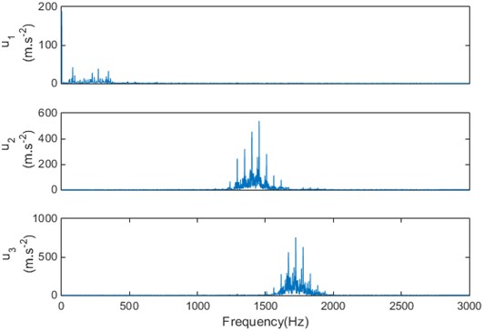
c) The spectrums of mode components when 3
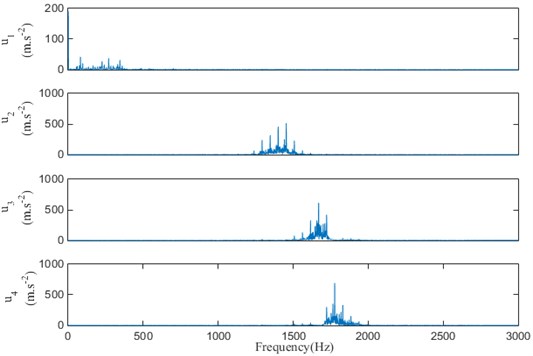
d) The spectrums of mode components when 4
It can be seen that when 2, the frequency band 1000 Hz-1500 Hz are mostly discarded, so it has a lack of information. When 4, the central frequencies of the modal components and are close to each other, it may cause the frequency aliasing. Therefore, the modal decomposition number is determined as 3. And according to the experimental debugging, the penalty parameter is set to 1000.
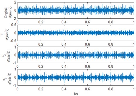
After the decomposition of each sample in the experimental dataset, three components containing the fault information are obtained. The original signal of inner ring fault and three modal components obtained by IVMD method are given in Fig. 10.
Then, normalize all the decomposition data, and label them with the one-hot structure. The whole dataset is divided into training dataset and test dataset, which are shown in Table 1.
Table 1Rolling bearing data set
Bearing states | Number of training samples | Number of test samples | Label of samples |
Normal | 750 each | 750 each | 1 |
Three different degrees of inner ring fault | 750 each | 750 each | 2/3/4 |
Three different degrees of outer ring fault | 750 each | 750 each | 5/6/7 |
Three different degrees of rolling element fault | 750 each | 750 each | 8/9/10 |
Fig. 10VMD results of bearing vibration signal with inner race fault
5.3. Design of DCNN model
The structural parameters of the designed DCNN model after repeated experiments and debugging are shown in Table 2. CS represents the size of convolution kernel. CN represents the depth of convolution kernel. I denotes the number of input graphs. Strides represents the step length of convolution kernel movement. S represents the width of pooling layer. FS1 and FS2 represent the size of the first and second full connection layers, respectively.
Table 2Parameters of DCNN structure
Structure | Parameter |
Convolution layer | CS = 1×32; CN = 64; I = 3; Strides = 1 |
Pooling layer | S = 4 |
Convolution layer | CS = 1×16; CN = 64; I = 64; Strides = 1; |
Pooling layer | S = 4 |
Convolution layer | CS = 1×4; CN = 128; I = 128; Strides = 1; |
Pooling layer | S = 4 |
Convolution layer | CS = 1×4; CN = 256; I = 256; Strides = 1 |
Pooling layer | S = 4 |
Full connection layer | FS1= 5×512; FS2= 10; Activation function: ReLU |
Softmax | The number of output nodes: 10 |
RMSProp | 0.001 |
RMSProp algorithm is adopted to optimize the DCNN model, and the global learning rate is set as 0.001. To prevent overfitting, dropout strategy and L2 regularization algorithms are adopted, with coefficients of 0.5 and 0.0012. In this way, the generalization performance of DCNN model is highly improved.
5.4. Analysis of experimental results
A total of 7500 samples in the training set are input into the designed DCNN model. Fig. 11 displays the change of the loss function values of the training set. When the model training reaches 2100 times, the loss function no longer changes significantly, which means that the model training is completed at this time. After multiple iterations, the training accuracy of the model is 100 % and the average diagnostic accuracy in the test set is 99.5 %.
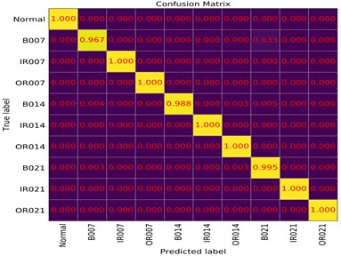
In order to present the diagnostic results of the model in the test set in more detail, a confusion matrix is introduced to analyze the experimental results. In Fig. 12, B007, B014 and B014 represent the rolling element fault with the fault size of 0.07 in, 0.14 in and 0.21 in, respectively.
Except that the diagnostic accuracy of rolling element fault with the fault size of 0.07 in is 96.7 %, identification accuracies of other 9 states is higher than 98.8 %, which indicates that this method can effectively realize the intelligent bearing fault diagnosis and obtain a high diagnostic accuracy.
Meanwhile, in order to compare the advantages of the proposed method in fault diagnosis, the above experimental data is also decomposed by EEMD method, where the intensity of white noise and the number of cycles are respectively set to Nstd = 0.3 and NE = 100. Then, the first three modal components with large kurtosis constitute a data sample set. In the light of Table 2, the data sets processed by EEMD are divided in the same way. Using the training dataset to train the DCNN model. Finally, the diagnosis accuracy of test dataset is 95.07 %.
From the above comparison, it can be seen that the proposed method based on IVMD and DCNN has a higher diagnostic accuracy, indicating that the IVMD algorithm can enhance the fault characteristics more effectively.
Fig. 11Loss function curve for training set
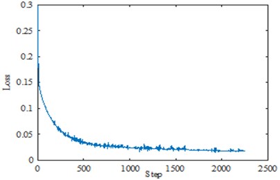
Fig. 12Diagnostic result of test dataset
5.5. t-SNE visual analysis
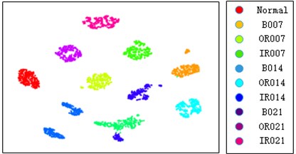
In order to more intuitively illustrate the adaptive feature learning ability of the DCNN model designed in this paper, t-SNE algorithm [20] is adopted to visualize the features learned from the first layer of the full connection layer of the DCNN model. The test samples are input into the trained DCNN model, and the feature distribution is shown in Fig. 13.
Each color in Fig. 13 represents a fault type, and the features in each state learned by the model are highly separated. The visualization results further show that the DCNN model can adaptively learn different state characteristics from the bearing vibration data after IVMD processing, and thus has a good fault classification capability.
Fig. 15Feature visualization
5.6. Comparison with other deep learning methods
In order to validate the effectiveness and superiority of the proposed method, the proposed method based on DCNN is further compared with other deep learning-based fault diagnosis methods, including deep belief network (DBN), sparse autoencoder (SAE) and one-dimensional CNN (1-D CNN) [21]. In every method, the same dataset is adopted. The structure of the DBN is 27-100-50-10. Its learning rate is 0.1, and the number of iterations is 400. SAE contains three hidden layers, each of which has a structure of 100-60-10. The learning rate is 0.2, and the number of iterations is 200. Structural parameters of 1-D CNN are just similar to those in literature [21]. In all these comparative models, learned signal characteristics are classified by softmax classifier. In order to eliminate the influences of randomness, each algorithm is repeated 20 times. Fault diagnosis results of these methods are summarized in Table 3.
Table 3Diagnosis results of different models
Method | Mean accuracy | Standard deviation |
DBN | 97.78 % | 1.3251 |
SAE | 96.93 % | 1.5345 |
1-D CNN | 99.15 % | 1.2034 |
The proposed method | 99.5 % | 0.0251 |
Compared with DBN and SAE models, the proposed method using DCNN model has the highest diagnostic accuracy and lowest standard deviation. Meanwhile, compared with the proposed DCNN-based method, the 1-D CNN model applied in literature [21] only has two convolution layers. Although its recognition rate reaches 99.15 %, it’s still lower than the proposed method. Moreover, the standard deviation of diagnosis results is much higher than the proposed DCNN model. These results proves that the DCNN model with deeper structure can improve the accuracy and stability of diagnosis results.
6. Conclusions
In this paper, aiming at the non-stationarity characteristic of the vibration signal of rolling bearings, a bearing fault diagnosis method based on IVMD and DCNN is proposed. Using the advantages of VMD in non-stationary signal processing and DCNN’s strong adaptive learning ability, the proposed method can realize intelligent fault diagnosis of rolling element bearing effectively. In order to solve the problem that VMD usually needs to set the number of decomposition modes in advance, IVMD is developed where the decomposition number is determined according to the IF mean curve. On this basis, the IVMD algorithm is used to preprocess the data, and the decomposed modal components are used to construct a data set with more prominent fault characteristics, which improved the diagnostic effect of DCNN. Experimental results show that the proposed method can achieve 99.5 % accuracy in fault diagnosis, which is higher in diagnosis accuracy and better in robustness compared with diagnosis methods based on EEMD and methods based on other deep learning models including DBN, SAE, and 1-D CNN.
References
-
El-Thalji I., Jantunen E. A summary of fault modelling and predictive health monitoring of rolling element bearings. Mechanical Systems and Signal Processing, Vol. 60, Issue 61, 2015, p. 252-272.
-
Pajak M., Muślewski Ł., Landowski B., Grządziela A. Fuzzy identification of the reliability state of the mine detecting ship propulsion system. Polish Maritime Research, Vol. 26, Issue 1, 2019, p. 55-64.
-
Wang R., Wang C., Li J., et al. An intelligent fault diagnosis method of rolling element bearing based on acoustic imaging and Gabor wavelet transform. 25th International Congress on Sound and Vibration, Hiroshima, Japan, 2018, p. 2684-2691.
-
Grządziela A., Musial J., Muślewski Ł., Pajak M. A method for identification of non coaxiality in engine shaft lines of a selected type of naval ships. Polish Maritime Research, Vol. 22, 2007, p. 65-71.
-
Zhao H. Y., Wang J. D., Lee J., Li Y. A compound interpolation envelope local mean decomposition and its application for fault diagnosis of reciprocating compressors. Mechanical Systems and Signal Processing, Vol. 110, 2018, p. 273-295.
-
Huang N. E., Shen Z., Long S. R. The empirical mode decomposition and the Hilbert spectrum for nonlinear and non-stationary time series analysis. Proceedings of the Royal Society, Vol. 454, Issue 1971, 1998, p. 903-995.
-
Ricci R., Pennacchi P. Diagnostics of gear faults based on EMD and automatic selection of intrinsic mode functions. Mechanical Systems and Signal Processing, Vol. 25, Issue 3, 2011, p. 821-838.
-
Wu Z., Huang N. E. A study of the characteristics of white noise using the empirical mode decomposition method. Proceedings of the Royal Society A: Mathematical, Physical and Engineering Sciences, Vol. 460, Issue 2046, 2004, p. 1597-1611.
-
Li H., Liu T., Wu X., Chen Q. Application of EEMD and improved frequency band entropy in bearing fault feature extraction. ISA Transactions, Vol. 88, 2019, p. 170-185.
-
Dragomiretskiy K., Zosso D. Variational mode decomposition. IEEE Transactions on Signal Processing, Vol. 62, Issue 3, 2014, p. 531-544.
-
Jiang X., Wang J., Shi J. A coarse-to-fine decomposing strategy of VMD for extraction of weak repetitive transients in fault diagnosis of rotating machines. Mechanical Systems and Signal Processing, Vol. 116, 2019, p. 668-692.
-
Li J. M., Yao X. F., Wang H., Zhang J. F. Periodic impulses extraction based on improved adaptive VMD and sparse code shrinkage denoising and its application in rotating machinery fault diagnosis. Mechanical Systems and Signal Processing, Vol. 126, 2019, p. 568-589.
-
Jiang W. L., Wang H. N., Zhu Y. Integrated VMD denoising and KFCM clustering fault identification method of rolling bearings. China Mechanical Engineering, Vol. 28, Issue 10, 2017, p. 1215-1220.
-
LeCun Y., Bengio Y., Hinton G. Deep learning. Nature, Vol. 521, Issue 7553, 2015, p. 436-444.
-
Badrinarayanan V., Kendall A., Cipolla R. SegNet: a deep convolutional encoder-decoder architecture for image segmentation. IEEE Transactions on Pattern Analysis and Machine Intelligence, Vol. 39, Issue 12, 2017, p. 2481-2495.
-
Wen L., Li X., Gao L. A new convolutional neural network based data-driven fault diagnosis method. IEEE Transactions on Industrial Electronics, Vol. 65, Issue 7, 2018, p. 5990-5998.
-
Jia F., Lei Y. G., Lu N. Deep normalized convolutional neural network for imbalanced fault classification of machinery and its understanding via visualization. Mechanical Systems and Signal Processing, Vol. 110, 2018, p. 349-367.
-
Peng D. D., Liu Z. L., Wang H. A novel deeper one-dimensional CNN with residual learning for fault diagnosis of wheelset bearings in high-speed trains. IEEE Access, Vol. 7, 2019, p. 10278-10293.
-
Case Western Reserve University Bearing Data Center Bearing data file [EB/OL], https//csegroups.case.edu/bearingdatacenter/ho-me.
-
Maaten L., Hinton G. Visualizing data using t-SNE. Journal of Machine Learning Research, Vol. 9, 2008, p. 2579-2605.
-
Ince T., Kiranyaz S., Eren L., Askar M., Gabbouj M. Real-time motor fault detection by 1-D convolutional neural networks. IEEE Transactions on Industrial Electronics, Vol. 63, Issue 11, 2016, p. 7067-7075.
About this article

This work was supported by the National Natural Science Foundation of China (Grant No. 51505277).
