Extraction and diagnosis of rolling bearing fault signals based on improved wavelet transform

3.1. Design of IEWT-RBF signal processing model based on normalization processing

RB in the normal working process will produce vibration because of the surface roughness, size deviation, etc. The signal issued by this vibration is normal smooth signal [16]. When the RBF point, rolling body and the fault point produce signal fluctuations, in a certain rotation speed, the corresponding fault frequency signal will be formed. This signal is not smooth and non-linear [17, 18]. Typical RB faults can be divided into three types: inner ring, outer ring, and ball bearing faults. The inner and outer rings are both circular parts that generate vibration when faults occur, and each of them only generates one fault frequency. Ball bearings are rolling parts inside bearings that come into contact with both the inner and outer rings simultaneously, resulting in two failure frequencies when a fault occurs. There is a certain difference between the diagnosis of inner and outer ring faults and the diagnosis of ball faults. Research is conducted to design methods for diagnosing inner and outer ring faults in RBs. EWT is a non-linear signal adaptive decomposition method, which can effectively attenuate the impact of modal confusion by applying in the RBF signal processing. The process of generating fault signals from RBFs is displayed in Fig. 1.

Fig. 1Process for generating fault signals of RBs

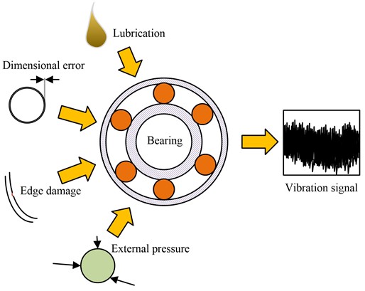
As seen in Fig. 1, RBF signals are generated by multiple factors. The natural working vibration of the RB itself and the vibration caused by dimensional deviation are the most basic vibrations. When lubrication conditions change and external pressure and bearing failure occur during operation, the vibration frequency and amplitude change and the output failure signal is hidden in the vibration signal. As the RB rotates, these signals are periodic. The vibration signal is first processed by the Fourier transform, and the resulting signal spectrum is normalized as shown in Fig. 2.

As seen in Fig. 2, the normalization process takes the half-perimeter rotation as a complete processing interval, and divides the interval into consecutive $N$ segments. ${\omega }_N$ is set as the center of each band, then ${\omega }_0$ and ${\omega }_n$ denote the upper and the lower boundary of the interval, respectively, and the length of the transition band is $2{\tau }_n$. The empirical wavelet function is constructed as shown in Eq. (1):

where, ${\omega }_n$ denotes the lower boundary of the $n$ band; the value of $\gamma$ is less than 1. The empirical scale function is constructed as shown in Eq. (2):

where, $\gamma$ is less than the ratio of the difference between the upper and lower boundaries of the frequency band to the sum of them. The definition of the modal component is shown in Eq. (3):

where, $W_f^{\epsilon }(n,t)$ means the detail coefficients, which are generated by the wavelet function and the signal inner product; $W_f^{\epsilon }(0,t)$ indicates the approximation coefficients, which are produced by the scale function and the signal inner product; ${\varphi }_1$ denotes the empirical scale coefficients. The output vibration signal is reconstructed as shown in Eq. (4):

where, ${\widehat{W}}_f^{\epsilon }(0,\omega )$, ${\widehat{W}}_f^{\epsilon }(n,\omega )$ are the Fourier transform of $W_f^{\epsilon }(0,t)$, $W_f^{\epsilon }(n,t)$, respectively. To perform the spectrum differentiation, the spectrum is divided into $N$ bands, and each band exists independently, excluding the two end points of the interval, and it also needs to determine the boundary points of $N-1$. The discrete scale space of the spectrum within a single interval is determined by the number of minima, and the function for calculating the number of minima is shown in Eq. (5):

where, $x$ is the variable; $t$ means the scale parameter; $g(n,t)$ indicates the Gaussian kernel function. When the RB is in a harsh working environment, the factors affecting the vibration become more and the generated vibration signal is more complex, and a large number of redundant and meaningless frequency bands will be generated when the frequency band is divided, which affects the subsequent RBF signal extraction efficiency. To improve the efficiency of fault signal extraction, Otsu is used to optimize the EWT process, and the IEWT transformation process is obtained, as shown in Fig. 3.

Fig. 2Spectrum processing diagram

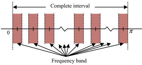
Fig. 3IEWT transformation process

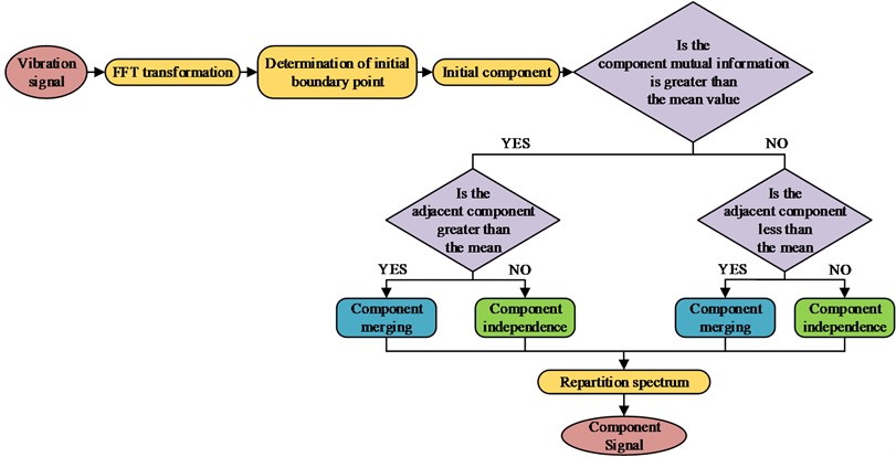
As seen in Fig. 3, the IEWT transform processes based on Otsu are as follows. First, it performs FFT transform on the input signal, and analyzes the Fourier spectrum. Then, the scale space curve threshold is determined by the Otsu method, and the initial dividing point is derived. It decides whether to merge the components according to their mutual information and the values of adjacent components, updates the Fourier spectrum according to the merged components, and outputs the optimized component signal [19, 20]. The vibration characteristics at the beginning of the RBF are weak and easily disturbed by other environmental noise when extracted. The vibration signal function of RBF is established as shown in Eq. (6):

where, $y\left(n\right)$ refers to the output signal; $x\left(n\right)$ denotes the input signal; $h\left(n\right)$ is the signal transfer function; and $e\left(n\right)$ represents the environmental noise. The smaller the entropy recovered to $x\left(n\right)$, the less the fault information is disturbed [21]. The value of $x\left(n\right)$ is taken as shown in Eq. (7):

where, $l$ represents the inverse filter length. The size of the entropy value of $x\left(n\right)$ is measured by the target parametrization of $x\left(n\right)$, and the objective function is established as expressed in Eq. (8):

where, $o_2^4\left(f\right(n\left)\right)$ is the parametric amount of $x\left(n\right)$. The partial derivatives of the entropy value and the parametric objective function are coupled as shown in Eq. (9):

where, $B$ is the inter correlation matrix of the input and output data obtained from the association; $g$ denotes the inverse filter matrix obtained from the iterative calculation; $A$ stands for the $L\times L$ autocorrelation matrix of the signal $y\left(n\right)$.

3.2. Optimized design of IEWT RBF signal extraction and diagnosis model based on SVM and QGA

After completing the pre-processing of the vibration signal of RBF, subsequent extraction of the fault signals is required to enter the diagnosis process. The study optimizes and reconstructs the RBF diagnosis process after the introduction of MED [22]. The optimized RBF diagnosis process is shown in Fig. 4.

Fig. 4Optimized RBF diagnosis process

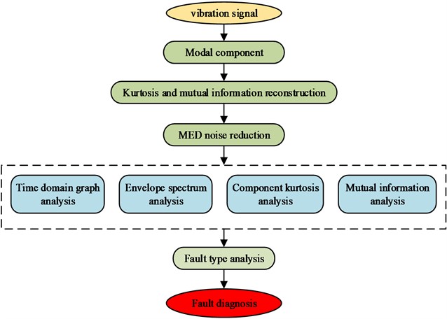
In Fig. 4, the optimized RBF diagnosis firstly separates the noise and impulse components from the fault information to obtain the modal component signal. After that, the modal component information is reconstructed using the peakness and mutual information criterion, and the components with the largest mutual information and those with too small peakness are excluded in the reconstruction. After obtaining the optimal modal components, the MED is used for noise reduction. The output vibration signal is analyzed in various aspects, and the data integration is completed. Finally, the fault diagnosis results are obtained. In the real working condition, it is not easy to sample the RBF, and the sample size of the fault signals that can be obtained is small, so the conclusions obtained by using traditional statistical analysis methods often have large deviations. SVM has good generalization ability when identifying and classifying, and has better anti-interference ability under small sample data, so it can be utilized to RBF diagnosis to improve the diagnosis accuracy [23]. The SVM works as shown in Fig. 5.

Fig. 5SVM classification plane

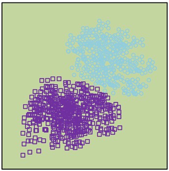
a) Initial classification plane

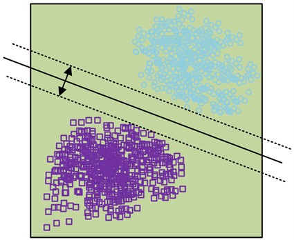
b) Insert optimal classification plane

In the basic case, SVM sets an optimal classification plane between two types of data point groups by analyzing the data points. It also inserts the optimal classification plane to squeeze the two types of data points towards both sides, and expands the classification interval, thus distinguishing the two types of data. The data are thus completely separated. The definition of the optimal hyperplane is shown in Eq. (10):

where, $x_i$ represents the input feature vector; $y_i$ indicates the sample category; $\omega$ means the weight vector; and $b$ means the bias vector. The classification interval is shown in Eq. (11):

where, $margin$ represents the classification interval value. The larger the classification interval is, the better the data points are classified, and the optimal classification plane selection is transferred to quadratic convexity, as shown in Eq. (12):

where, $a_i$ is the introduced $Lagrange$ multiplier. The decision function of the optimal classification plane is shown in Eq. (13):

where, $f\left(x\right)$ represents the optimal classification plane decision function, which is derived from the optimal classification plane solution by quadratic search for the best solution. When nonlinear data are involved, the introduction of the kernel function can map the features to a high-dimensional space, thus transforming the nonlinearly indistinguishable data into linearly distinguishable data in a high-dimensional space. The pairwise problem $Lagrange$ is transformed as shown in Eq. (14):

where, $c$ is a constant. The decision function of the nonlinear SVM undergoes a transformation, as shown in Eq. (15):

where, $y_k$ represents the sample category; $\mathrm{s}\mathrm{g}\mathrm{n}\left\{\right\}$ is the symbolic function. The Gaussian radial basis kernel function is utilized as the kernel function, as shown in Eq. (16):

where, $\sigma$ expresses the kernel parameter, and the smaller the kernel parameter, the better the learning ability of SVM. The ranking entropy is able to analyze the dynamic changes of the signal by integrating the temporal connections between data points, and the entropy value is calculated without setting the probability distribution of the signal in advance. The definition of the ranking entropy is expressed in Eq. (17):

where, $H_p\left(m\right)$ is the definition of alignment entropy according to the Shannon entropy setting; $k$ represents the number of reconstruction vectors; $\mathrm{l}\mathrm{n}(m!)$ is the maximum value obtained by $H_p\left(m\right)$ under the condition of $p_l=1/m!$; the value of $H_p$ takes the range of $0\le H_p\le 1$, the smaller the value is, the weaker the randomness of the time series and the lower the sequence complexity. The values of optimal kernel parameter width and penalty coefficient affect the accuracy and generalization ability of SVM. Too large a kernel parameter width or too small a penalty coefficient will lead to insufficient classification accuracy; too small a kernel parameter width or too large a penalty coefficient will lead to insufficient generalization ability of SVM [24]. Using QGA for parameter selection can improve the efficiency of optimal parameter selection. The flow of optimal parameter selection using QGA is shown in Fig. 6.

Fig. 6Optimal parameter selection process based on QGA

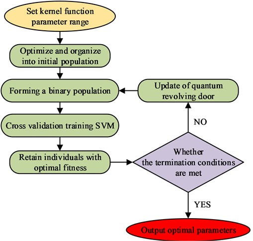
As seen in Fig. 6, for parameter selection, the number of populations, the maximization algebra, and the range of penalty coefficients need to be determined first. Then, the populations are initialized and binary measurements are transformed into binary string codes. The randomly generated parameter combinations are input to the SVM for processing, cross-validation training is performed, and the resulting best parameter combinations are retained. The search is continuously verified using a quantum revolving gate until the fitness function satisfies the termination condition and the resulting best optimized parameters are output. The initial population is shown in Eq. (18):

where, $N$ represents the number of randomly generated chromosomes; $P_n^t$ denotes the first $n$ individual that evolves to the $t$ generation; $P\left(t\right)$ is encoded by quantum bitwise. The quantum revolving door search is shown in Eq. (19):

where, $U\left({\theta }_i\right)$ is the revolving door operation; ${\theta }_i$ represents the rotation angle. The RB fault feature extraction and diagnosis model designed by this research integrates multiple methods to achieve the fusion of multimodal features, which can capture RB fault information from different dimensions and scales. By introducing QGA, representative features can be adaptively selected, and redundant information can be eliminated. Compared to traditional methods that combined wavelet transform with SVM, it has better diagnostic efficiency. When conducting fault diagnosis, research methods can provide a certain degree of interpretability for the diagnostic process and results. In practical applications, compared to general wavelet transform methods, they have better applicability and can reduce the information burden on engineering personnel.

4.1. Performance test of IEWT-SVM based RBF signal extraction and diagnosis model

To verify the effectiveness of the IEWT-SVM-based RBF signal extraction and diagnosis model at runtime, the study first tested the performance of the constructed diagnosis model. During the test, the data used in the experiment came from the bearing database of the electrical laboratory of Case Western Reserve University in the United States. This database is the most commonly used data set in the field of RB fault diagnosis, which belongs to the standard data set. The data of 6205-2RS JEM SKF deep groove ball bearing at the drive end of the database were selected for calculation, with the sampling frequency of 12 kHz. The sampling frequency of the simulation signal was set to 20 kHz. The damping coefficient was 0.1. The displacement constant was 5. The natural frequency was 3 kHz. The rotation frequency was 25 Hz. The impact amplitude was 1.2 m/s². The noise amplitude was 3.0 m/s². The harmonic amplitude was 1.5 m/s². The attenuation rate was 800. The inner ring diameter of the experimental bearing was 25 mm. The outer ring diameter was 52 mm. The pitch diameter was 39.04 mm. The diameter of the ball is 7.94 mm. The number of rolling balls was 9. The contact angle was 90°. Two faults were set in the rolling element, with dimensions of 0.1778 mm and 0.3556 mm, respectively. When conducting application analysis, a double row roller bearing with model FAG F-80781109 TAROL 130/240-B-TVP was used, and a fault groove with a length of 5 mm, a depth of 0.7 mm, and a width of 1 mm was manufactured using electric spark. The fault experimental system used is shown in Fig. 7.

Fig. 7Fault experimental system

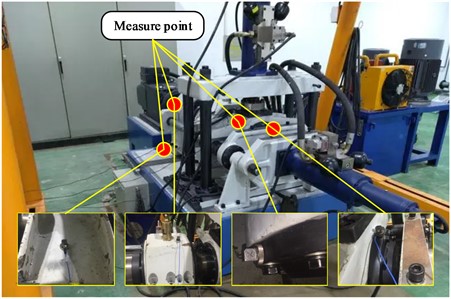
As shown in Fig. 7, the experimental system used was established on a high-speed train bearing experimental platform, where sensors were installed at different positions to collect data. The high-speed train bearing experimental platform was set to rotate at 1200 revolutions per minute. When conducting experiments, wavelet transform was performed on data in different states, retaining the first five modal components, and then the arrangement entropy was calculated to obtain the input feature vector set. The content of system performance testing included dividing spectrum performance testing and simulating signal time-domain diagrams. After completing parameter optimization and training, the envelope spectrum, component kurtosis, diagnostic accuracy, and component diagnostic results would be used as application analysis content. The study first tested the performance of EWT and IEWT-SVM for dividing the spectrum, and the test results are shown in Fig. 8.

Fig. 8Divide spectral images

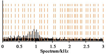
a) EWT original partition spectrum

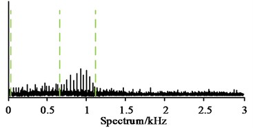
b) IE WT-SVM repartition spectrum

As seen in Fig. 8(a), in the same spectrum interval, IEWT divided the interval into 37 bands according to the band anomalies, and each band was short in length and contained less information. Some bands divided the same anomaly into multiple small bands, which also generated more meaningless bands. In Fig. 8(b), IEWT-SVM determined a new cut-off point according to the overall trend, and divided the interval into four frequency bands according to the new cut-off point and the anomalies, preserving the integrity of each anomalous band and effectively reducing the generation of redundant bands. The time domain diagrams of the simulated signals in the same time period were compared, and the results are shown in Fig. 9.

Fig. 9Time domain diagram of simulated signal

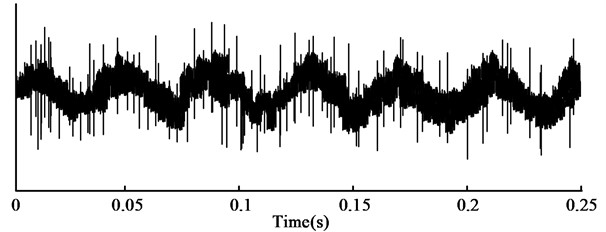
a) EWT time domain diagram of simulated signal

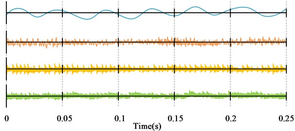
b) IE WT-SVM component signal time-domain diagram

As seen in Fig. 9(a), a complete time domain map containing all the information was obtained by IEWT in the 0-0.25 s time period, in which the overall trend and fluctuation of the signal could be roughly distinguished, but the specific composition of the signal and the amplitude of each component could not be judged intuitively. In Fig. 9(b), IEWT separated the simulated signal and obtained four component simulated signals. The harmonic, shock and noise components were separately represented, and the trend and variation of each component could be judged more intuitively. It indicated that IEWT-SVM could effectively extract the abnormalities in the signal when performing RBF signal extraction and diagnosis, and could output better diagnosis data.

4.2. Analysis of the application effectiveness of IEWT-SVM based RBF signal extraction and diagnosis model

The envelope spectrum of the wheel-to-wheel bearing containing the inner ring spalling fault was extracted, and the envelope spectrum generated by using ordinary spatial noise reduction was compared with that generated by IEWT-SVM, and the results are shown in Fig. 10.

Fig. 10Envelope spectrum after noise reduction

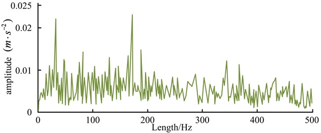
a) Normal space noise reduction

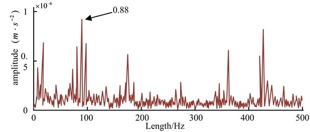
b) IEWT-SVM

In Fig. 10(a), the overall amplitude of the envelope spectrum generated by normal spatial noise reduction was low in the 500 Hz length, with the highest value below 0.25 (m⋅s^-2). The amplitude fluctuation was obvious, but the obtained spectrum fluctuated frequently, leading to confusion between some normal high amplitude values and abnormal amplitude values around 0.01 (m⋅s^-2). In Fig. 10(b), the overall amplitude of the envelope spectrum generated by IEWT-SVM was also low. After the noise reduction optimization process, some of the highest amplitude values reached 0.88×10^-6 and the abnormal amplitude values basically reached above 0.40×10^-6, which had obvious high and low differences with the normal amplitude values and could distinguish the abnormal amplitude values from the normal amplitude values more effectively. It was also necessary to generate the peak value to derive the reconstructed signal when judging the fault, and the ensemble empirical mode decomposition (EEMD) was compared with the component peak situation generated by IEWT-SVM, and the results are shown in Fig. 11.

Fig. 11Ensemble empirical mode decomposition (EEMD) vs with the component peak situation generated by IEWT-SVM

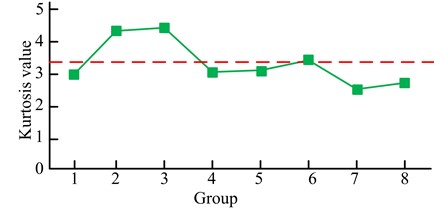
a) EEMD

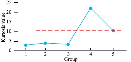
b) IEWT-SVM

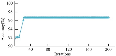
In Fig. 11(a), EEMD generated 8 component quantitative peaks with the maximum peak of 4.4533 and the minimum peak of 2.6853, and finally output 3 components that were larger than the average value of 3.3766. As seen in Fig. 11(b), IEWT-SVM generated 5 component quantitative peaks, with the maximum peak of 22.1611 and the minimum peak of 2.7686. Finally, it output 1 component quantitative peak with the maximum peak, which could reduce the pressure of subsequent data processing and improve efficiency. The kernel function width and penalty coefficients were iteratively searched for using SVM-based GA and IEWT-SVM, and the accuracy of RBF diagnosis was derived using the obtained kernel function width and penalty coefficients, and the outcomes are shown in Fig. 12.

Fig. 12Iterative optimization results

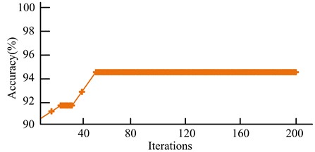
a) GA

b) IEWT-SVM

As seen in Fig. 12(a), the GA reached the highest accuracy after 50 iterations out of 200 iterations, with a short rising stagnation between the 20th and 30th iteration intervals, with an initial accuracy of 90.4 % and a final stable maximum accuracy of 94.6 %. As seen in Fig. 12(b), the IEWT-SVM reached the highest accuracy after 24 iterations out of 200 iterations, with a short rising stagnation between the 3rd and 10th iteration intervals and a final stable maximum accuracy of 96.7 %. It indicated that IEWT-SVM had better iteration speed and judgment accuracy. The results were shown in Fig. 13, using GA, Particle Swarm Optimization (PSO) method and IEWT-SVM for component diagnosis under the generated optimal kernel function width and penalty coefficients, and three sample labels were set for diagnosis.

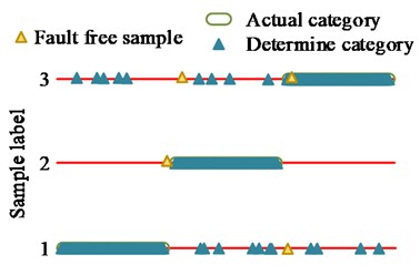
Fig. 13Component diagnosis results

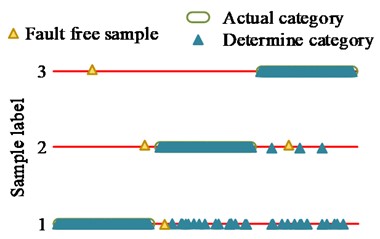
a) GA

b) PSO

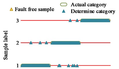
c) IEWT-SVM

When conducting component diagnosis, all three methods classified faulty and faultless samples. From Fig. 13(a), during component diagnosis by GA, there were no misjudgments for the classification that originally belonged to the first class label results, but some samples of the second and third class labels were mistakenly classified into the first class label. In the classification results, there were 4 errors in selecting faultless samples, and the overall judgment accuracy was 90.33 %. From Fig. 13(b), when PSO performed component diagnosis, there was a certain amount of misjudgment in the results of various label samples, but the overall number was less than GA. In the classification results, there were three errors in selecting faultless samples, with an overall accuracy rate of 94.33 %. From Fig. 13(c), IEWT-SVM mistakenly classified a small number of samples belonging to the first class label into the third class label during component judgment, and mistakenly classified a small number of samples belonging to the second class label into the first and third class labels. The classification that originally belonged to the third class label results did not show any misjudgment, and the overall judgment accuracy was 98.12 %. When using research methods for diagnosis, fault samples were more accurately detected, and the proportion of fault samples accurately classified into labels was higher. It denoted that the research method had better model sensitivity and detection accuracy, and the probability of misjudgment was lower. When label classification was performed on faulty samples, only faulty samples were classified, and all faultless samples were excluded, indicating good specificity of the research method.