Rolling bearing fault diagnosis with compressed signals based on hybrid compressive sensing

In recent years, many studies have been conducted on remote machine condition monitoring and on-board bearing fault diagnosis. To accurately identify the fault pattern, large amounts of vibration data must be sampled and saved. However, because the bandwidth of the wireless communication is limited, the volume of transmitted data cannot be too large. Therefore, raw data are usually compressed before transmission. All of the previous compression methods use a sample-then-compress framework; however, in this work, we introduce a compression method based on a Compressive Sensing that can simultaneously collect and compress raw data. Additionally, a hybrid measurement matrix is designed for Compressive Sensing and used to compress the data and make it easy to conduct fault diagnosis in the compression domain. This process can significantly reduce the computational complexity of on-board fault diagnosis. The experimental results demonstrate that the proposed compression method is easy to use and the reconstruction process can recover the original signal perfectly. Above all, the compressed signal can preserve the time series information of the original signal, and in contrast to fault diagnosis using the original signal, the accuracy of the fault diagnosis based on conventional methods in the compression domain is not significantly decreased.

1. Introduction

Rolling bearings are widely used in a number of different industries. Fault diagnosis is a useful method for increasing the reliability and performance of the rotating components of rolling bearings. In rotating machines, information is gathered by an acquisition system for use in the fault diagnostics system. The acquisition system must simultaneously sample vibrations or other signals through many channels at a high sampling speed to assure diagnostic accuracy. Therefore, the amount of raw data required for fault diagnosis is often massive. Thus, for fault diagnostic systems, especially for those online, as well as for remote fault diagnostic systems, it is necessary to save real-time data on hard disks for a long period of time, which can sometimes be difficult. Moreover, with the development of remote fault diagnostic techniques, high-performance data compression and reconstitution techniques are becoming increasingly popular, and these techniques will be useful for reducing the cost of large data transmissions and will further improve the performance of remote fault diagnostic systems. A compression algorithm is required for decompression; therefore, when a maintenance center receives compressed data, the center can ensure that the received data can be reconstructed into its temporal waveform and that as little information as possible is lost to maintain accurate fault diagnosis.

The existing signal compression methods can be categorized into four types: direct data compression methods, parameter extraction methods, transformation methods, and direct sparse representation compression methods.

Direct compression methods directly handle and compress the original data. Ref. [1] compares different direct compression techniques used for Electrocardiogram data. Parameter extraction methods design a pre-processor to extract features from the original signal first and then compress the signal based on the extracted features. For example, Ref. [2] presents a comparison between the performances of neural network and discrete cosine transform for near-lossless compression of EEG signals. Unfortunately, neural network based methods require a large amount of computing resources, which is difficult to achieve from a remote port. Transformation compression methods include Fast Fourier Transform (FFT) [3], wavelet transform (WT) [4], and Hilbert–Huang transform (HHT) [5]. In regard to rolling bearing fault diagnosis, the FFT-based methods are not suitable for the analysis of bearing vibration signals, which are always nonstationary signals. Ref. [6] studied the performance of the WT-based data compression methods for different types of signals; however, no general guidelines have been proposed for properly selecting a wavelet basis function. Incorrect use of wavelet base functions will lead to poor compact support and make wavelet coefficients sparse, making it difficult to achieve proper data compression. HHT is derived from the principals of empirical mode decomposition (EMD) and the Hilbert Transform method and is an adaptive signal processing method for analyzing nonlinear and non-stationary signals. However, the EMD process will generate undesirable intrinsic mode functions (IMFs) in the low-frequency region, and this process depends on the analyzed signal; therefore, the first obtained IMF may cover a frequency range that is too large and, consequently, may not contain the mono-component. Direct sparse representation compression methods employ an overcomplete dictionary of frequent occurring patterns. When these patterns appear in new signals, they are encoded with a reference to the dictionary. Ref. [7] uses a multiscale sparse dictionary to approximate seismic data. When sample data are in the remote port, direct sparse representation compression methods require complex calculations; however, for fast onboard signal acquisition systems and fault diagnosis systems, these methods are not very effective.

All of the previous compression methods use a sample-then-compress framework, which uses a K-sparse vector to represent the N-sample’s original signal $x$ . Unfortunately, this sample-then-compress framework has three inherent inefficiencies [8]. First, the initial number of samples $N$ may be large even if the desired $K$ is small. Second, the set of all $N$ transform coefficients must be computed even though all but $K$ of them will be discarded. Third, the locations of the large coefficients must be encoded, thus introducing overhead. To overcome these shortcomings, Donoho [9], Candes [10] and Tao introduced a Compressive Sensing (CS) theory that directly acquires a compressed signal representation, without going through the intermediate stage of acquiring $N$ samples, which means that signal sampling and compressing can now be achieved simultaneously. This characteristic reduces the amount of sampled data and is significantly different from previous methods. Therefore, data compression methods based on CS theory can simply compress the original data and reconstruct them perfectly in the maintenance center. Additionally, the hardware implementation of CS is simpler than previous techniques. As a practical example, consider a single-pixel, compressive digital camera that directly acquires $M$ ( $M ≪ N$ ) random linear measurements without first collecting the $N$ pixel values [11].

In recent years, many scholars combine deep learning with compressive sensing to design a variety of deep compressed sensing (DCS) neural networks. DCS generally includes block based DCS and frame based DCS. These researches apply convolutional neural network and other deep learning methods to the reconstruction algorithm of compressed sensing. DCS significantly improve the accuracy of data reconstruction, but the sampling part still uses the traditional compressive sensing method. For example, in reference [11], convolutional neural network is used for reconstruction, however its data compression part is still carried out using the random sensing matrix. Ref. [12] design sampling network, preliminary reconstruction network and deep reconstruction network. However, the essence of sampling network is still random sensing matrix, and the sampling network does not participate in the training. Therefore, this network is consistent with the traditional compressive sensing matrix.

In fault diagnosis research, we can consider Haile’s research [13], in which CS is used in structural health monitoring and the cost of collecting monitoring data is reduced. Furthermore, in Ref. [14], CS is combined with wireless sensor monitoring and is used in a coalmine. In these studies, monitoring data are analyzed after data recovery [15]; however, in rolling bearing fault diagnosis, it would be advantageous to manipulate the compression data in the measurement domain to reduce the computational resources consumption without data reconstruction. In this paper, a hybrid measurement matrix to compress the original data and make them easy to recover is designed. The advantage of this design is that the compressed data can reserve the time-frequency characteristics of the original data so that simple conventional methods can be used for fault diagnosis in the measurement domain. The experimental results show that this process not only significantly reduces the computational complexity in the remote data acquisition system but also the fault diagnostic accuracy is not significantly reduced. The trade-off of computational complexity and fault diagnostic accuracy can make a difference.

The remainder of this paper is organized as follows: In Section 2, the proposed method is described in detail in Section 3, the effectiveness of the proposed method is demonstrated with two experiences; and finally, conclusions are drawn in Section 4.

2. Methodology

The procedures of this study are shown in Fig. 1.

Fig. 1Architecture of the study

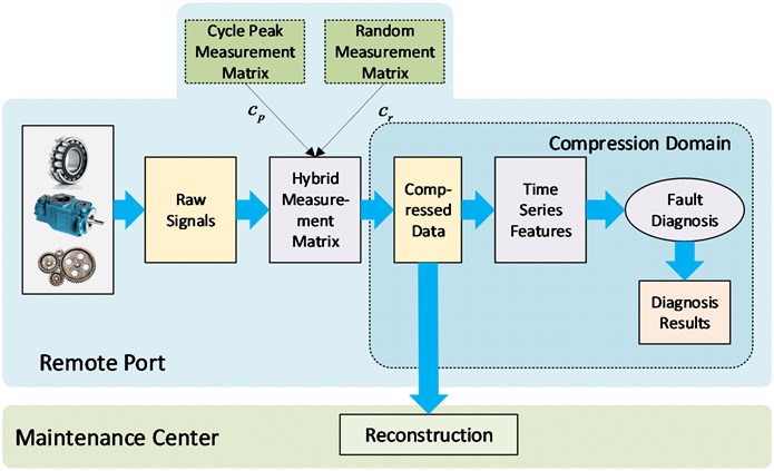
First, a hybrid measurement matrix is designed and used to accurately adjust the sensor of CS in the data acquisition system. Second, after the data acquisition system samples signals, the original signals can then be compressed through the hybrid measurement matrix. Third, in the remote port, the compressed signals retain the time series features of the original signals and conventional methods can be used to conduct fault diagnosis. Finally, the reconstruction algorithm can be used to recover the original signals in the maintenance center.

2.1. A brief introduction of the compressive sensing theory

This section gives a short introduction of CS theory. CS theory is a novel sensing/sampling paradigm that goes against common wisdom in data acquisition. CS is a new method to capture and represent compressible signals at a rate significantly below the Nyquist rate. In this method, many natural signals have concise representations when expressed in a convenient basis. In CS theory, similar to sparse representation, we assume that a signal can be sparse in some domain. A foundation for transform coding can be formed because the compressible signals are approximated well by K-sparse. Therefore, a one-dimensional signal $x$ in $R^{N}$ with length $N$ can be represented as:

1

x = Ψ θ,

where $Ψ$ is a $N \times N$ dictionary matrix, $θ$ is the coefficient sequence of $x$ , and there are only $K$ $(K ≪ N)$ coefficients that are nonzero in $θ$ .

The measurement process computes $M < N$ inner products between $x$ and a measurement matrix as:

2

y = Φ x,

where $Φ$ is a $M \times N$ matrix and $y$ is a $M \times 1$ vector; in other words, $y$ is a linear measurement or a condensed representation of $x$ .

Then, by substituting $Ψ$ from Eq. (1), $y$ can be written as:

3

y = Φ x = Φ Ψ θ = Θ θ .

In data acquisition systems, $Φ$ is fixed and does not depend on the signal $x$ . Through the data sampling process, we can obtain a compressed signal $y$ and then only transmit $y$ to the maintenance center. When the maintenance center receives the compressed signal $y$ , the process of recovering $x \in R^{N}$ from $y \in R^{M}$ starts. As we know, $x$ is K-sparse and a sufficient condition for a stable solution for both K-sparse and the compressible signal is defined by the measurement matrix $Φ$ and dictionary matrix $Ψ$ satisfying a restricted isometry property (RIP). The RIP can be achieved with high probability by simply selecting $Φ$ as a random matrix.

The last problem is to design a reconstruction algorithm to recover $x$ from $M$ measurements of $y$ only. The reconstruction algorithm aims to find the signal’s sparse coefficient vector $θ$ in the $(N - M)$ -dimensional translated null space. In general, the original signal $x$ is reconstructed from the compression signal $y$ using the following optimization process:

4

\hat{θ} = a r g m i n {‖θ‖}_{1} s . t . y = Θ θ,

where ${‖θ‖}_{1}$ is the $l_{1}$ norm of the vector $θ$ . This convex optimization problem conveniently reduces to a linear program known as basis pursuit (BP) [20] and orthogonal matching pursuit (OMP) [21]. This process can recover K-sparse signals exactly how they were and closely approximate the original signal $x$ with high probability by using only $M \geq c K l o g (N / K)$ independent and identically distributed (iid) Gaussian measurements.

2.2. Hybrid compressive sampling

In general, the measurement matrix of compressive sensing is a Gaussian matrix or another random matrix. Every row of the measurement matrix can be seen as a sensor and every sensor has a measurement from the original signal. When using a random matrix as the measurement matrix, each compressed signal value can be regarded as a weighted sum of values for each of the original signals. Therefore, the time series information of the original signal cannot be reserved in the compressed signal. In this paper, a hybrid measurement matrix is designed to compress the original data and allow the compressed signal to retain the time series information of the original signal; consequently, we can expediently use conventional methods for fault diagnosis in the measurement domain.

To make the compressed signal retain the original time series information, a cycle peak measurement matrix is designed such that every row has a $n_{p} (n_{p} = n / m)$ coefficient of 1, and the rest are 0. The location of these nonzero peaks in the $j$ -th row of the measurement matrix is $1 + (j - 1) \times n_{p}$ to $j \times n_{p}$ column. For example, if $n_{p} = 2$ then the cycle peak measurement matrix is:

5

[\begin{matrix} 1 & 1 & 0 & 0 & 0 & 0 & 0 & 0 & 0 & 0 & 0 & 0 \\ 0 & 0 & 1 & 1 & 0 & 0 & 0 & 0 & 0 & 0 & 0 & 0 \\ 0 & 0 & 0 & 0 & 1 & 1 & 0 & 0 & 0 & 0 & 0 & 0 \\ 0 & 0 & 0 & 0 & 0 & 0 & 1 & 1 & 0 & 0 & 0 & 0 \\ 0 & 0 & 0 & 0 & 0 & 0 & 0 & 0 & 0 & ⋱ & 0 & 0 \\ 0 & 0 & 0 & 0 & 0 & 0 & 0 & 0 & 0 & 0 & 1 & 1 \end{matrix}] .

Every row of the cycle peak measurement matrix can be regarded as a sensor, and the rows in the matrix are unrelated to each other, ensuring the effectiveness of the measurement. Cycle peak, in this paper, is defined as the peak of a square wave; however, it can also be the normal distribution. If this measurement matrix is used directly, the compressed signal can reserve the original time series information; however, the compressed signal cannot keep most of the information from the original signal. Therefore, the reconstruction effect is very poor. To correct this shortcoming, we introduce a hybrid measurement matrix consisting of a cycle peak matrix and a random matrix, as shown in Eq. (6):

6

Φ = c_{p} Φ_{p} + c_{r} Φ_{r},

where $Φ_{p}$ is a cycle peak matrix, $Φ_{r}$ is a Gaussian random matrix, $c_{p}$ is a time series property coefficient, and $c_{r}$ is a random property coefficient.

Based on this measurement matrix, the compressed signal can be used for fault diagnosis based on conventional diagnostic methods though the compression process.

2.3. Compressive feature extraction and fault classification

Recently, EMD has become a popular feature extraction method. The Support Vector Machine (SVM) is a simple and traditional fault diagnosis method. Here, two methods are introduced.

In the EMD process, the main function of EMD is to decompose the original signal into a series of IMFs ranging from high frequencies to low frequencies based on an iterative sifting process. Then, the IMF can represent the simple oscillatory mode in the signal, with the assumption that the signal consists of different simple intrinsic modes of oscillation (i.e., different simple IMF).

From the definition, the signal $x (t)$ is decomposed into $n$ intrinsic modes with a residue $r (t)$ :

7

x (t) = \sum_{i = 1}^{n} {I M F}_{i} (t) + r (t) .

Thus, the signal can be decomposed into $n$ -empirical modes with residue $r (t)$ , which is the mean trend of $x (t)$ .

EMD energy entropies of different signals illustrate that the energy of the signal is at different frequency bands that change when bearing fault occurs. To illustrate this change, the energy of each IMF is calculated.

The energies of the $n$ IMFs are $E_{1}, E_{2}, \dots$ respectively:

8

E_{i} = \int_{- \infty}^{+ \infty} {|{I M F}_{i} (t)|}^{2} d t, i = 1,2, \dots, n .

In ${[E}_{1}, E_{2}, \dots, E_{n}]$ vector, $E_{i}$ is arranged from high to low according to the value. We only saved a few components that accounted for more than 90 % of the total energy of $x (t)$ :

9

\sum_{n} E_{i} \geq 0.9 \times E (x) .

There are resonant frequency components created in the vibration signals of a bearing with different defects when it is running. The energy of the vibration signal fluctuates with the frequency distribution. As a result of the EMD decomposition being orthogonal, the sum of the n IMFs' energy should be equal to the total energy of the original signal if the residue $r (t)$ is disregarded. As the IMFs comprise multiple frequency components, ${[E}_{1}, E_{2}, \dots, E_{n}]$ creates a frequency domain energy distribution of bearing vibration signals.

To illustrate this change case as mentioned above, the EMD energy feature concept is defined as:

10

F = [E_{1} / E, E_{2} / E, \dots, E_{n} / E] .

$E$ is the 2-norm of ${[E}_{1}, E_{2}, \dots, E_{n}]$ :

11

E = \sqrt{E_{1}^{2} + E_{2}^{2} + \dots + E_{n}^{2}} .

In this paper, only the energies of the $m$ largest weights, as the features of original signals or compressed signals are saved.

An SVM is a classifier that is formally defined by a separating hyperplane. The operation of the SVM algorithm is based on finding the hyperplane that gives the largest minimum distance to the training examples.

A hyperplane is defined as:

12

f (x) = β_{0} + β^{T} x,

where $β$ is the weight vector and $β_{0}$ is the bias. For convenience, among all of the possible representations of the hyperplane, the hyperplane that is chosen is:

13

|β_{0} + β^{T} x| = 1,

where $x$ symbolizes the training examples closest to the hyperplane. In general, the training examples that are closest to the hyperplane are called support vectors. This representation is known as the canonical hyperplane.

The distance between a point $x$ and a hyperplane is:

14

D = \frac{|β_{0} + β^{T} x|}{‖β‖} = \frac{1}{‖β‖} .

The margin, denoted as $M$ , is twice the distance to the closest examples:

15

M = \frac{2}{‖β‖} .

Finally, the problem of maximizing $M$ is equivalent to the problem of minimizing a function $L (β)$ subject to some constraints. The constraints model for the requirements of the hyperplane are used to correctly classify all of the training examples $x_{i}$ . Formally:

16

\min_{β, β_{0}} L (β) = \frac{1}{2} {‖β‖}^{2} s . t . y_{i} (β_{0} + β^{T} x_{i}) \geq 1,

where $y_{i}$ represents each of the labels of the training examples. This is a Lagrangian optimization problem that can be solved using Lagrange multipliers to obtain the weight vector $β$ and the bias $β_{0}$ of the optimal hyperplane.

3. Experimental results

The bearing data used in this paper are taken from the Case Western Reserve University Bearing Data Center. The data consist of one set of normal bearing data and three common types of bearing defects (i.e., inner race defect, ball defect, and outer race defect). Defects ranging from 0.007 to 0.040 inches in diameter are identified at the inner raceway, rolling element (i.e., ball), and outer raceway separately. The motor speed is 1750 r/min, and the sampling rate is 12 kHz. Vibration data was collected using accelerometers, which were attached to the housing with magnetic bases.

Each pattern is induced in 36 samples and tested in 12 samples; every example has 2048 points where the vibration signal is determined. For classification purposes, the four patterns are marked as one, two, three, and four. The training matrix used is $R^{2048 \times 144}$ , and the column arrangement can be seen in Table 1. The testing matrix used is $R^{2048 \times 48}$ , and the column arrangement can be seen in Table 2.

Table 1Training matrix arrangement

Column number	1-36	37-72	73-108	109-144
Pattern	Normal	Inner race defect	Ball defect	Outer race defect

Table 2Testing matrix arrangement

Column number	1-12	13-24	25-36	37-48
Pattern	Normal	Inner race defect	Ball defect	Outer race defect

In this study, two experiments are conducted. In the first experiment, a hybrid measurement matrix is used to compress the original bearing data and reconstruct it based on OMP. In the second experiment, a fault diagnosis is conducted based on the compressed signal in the measurement domain. A comparison of the fault diagnosis is conducted based on the original data and the compressed signal and discussed in detail.

The measurement matrix used in all experiments is a hybrid compression matrix consisting of a cycle peak matrix $Φ_{p} \in R^{1024 \times 2048}$ and a Gaussian random matrix $Φ_{r} \in R^{1024 \times 2048}$ . Normally, we can set empirical parameter $c_{p} = 1$ then $c_{r}$ can be a smaller value that means $c_{r} < 0.05 \times c_{p}$ . In this paper we use $c_{r} = 0.018$ :

17

Φ = Φ_{p} + 0.018 \times Φ_{r} .

These matrices are expressed in the form of a grayscale image. Below, Fig. 2 shows the cycle peak matrix, and Fig. 3 shows the Gaussian random matrix.

In this paper, we set $M =$ 1024 and $N =$ 2048, so the compression ratio is 50 %. When using the proposed method, we can save half of the storage space.

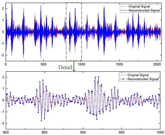
3.1. Comparison of the original signal and the reconstructed signal

In this experiment, the original bearing signal is compressed and reconstructed. The measurement matrix used is a hybrid measurement matrix, the dictionary matrix is a Fourier matrix, and the reconstruction algorithm used is OMP.

The normal signal and inner race defect signal are shown as examples below. Fig. 4 represents the normal signal and Fig. 5 represents the inner race defect signal, where the red lines are the original signals and the blue lines are the reconstruction signals.

Fig. 2Cycle peak matrix

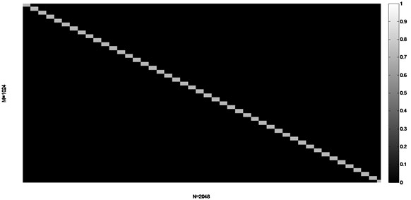
Fig. 3Gaussian random matrix

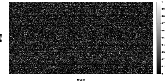
Fig. 4The reconstruction of the normal signal

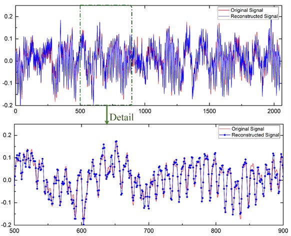
The results show that the original signal and the reconstruction signal are very similar. The reconstruction achieved an average normalized absolute error of 5.3 %. These results suggest that we can use the reconstruction signal to conduct further diagnosis and assessment in the maintenance center.

Fig. 5The reconstruction of the inner race defect signal

3.2. Fault diagnosis measurement based on the compressed signal

To verify whether the hybrid compression matrix could retain the time series of the original signal, EMD is used to obtain the time-frequency characteristics of the compressed signal.

Fig. 6IMF

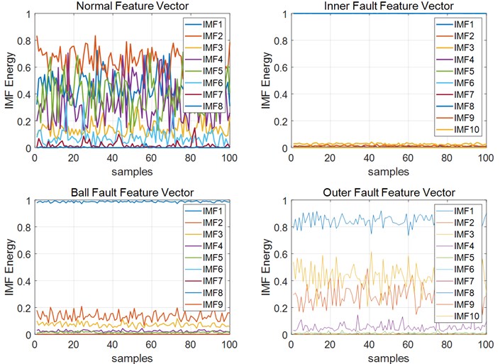
First, the original vibration signals were decomposed into some IMFs by EMD. The IMF vectors of every signal had different dimensionality because EMD can self-adaptive decompose signals, as shown in Fig. 6. It is clearly shown that only the first several IMFs had dominant fault information. According to Eq. (9), we saved the first nine IMFs.

Through the EMD process, we only save the first nine IMFs and use the energy of these IMFs as a signal feature. Therefore, the energy-training matrix used is a 9×144 matrix. For simplicity and visualization, only the maximum three energies of each training sample are retained. The new energy-training matrix is a 3×144 matrix, as shown in Fig. 6.

Fig. 7Compressed signal features

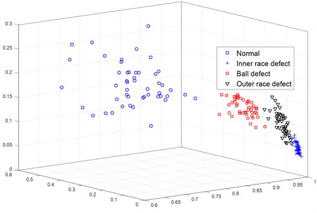
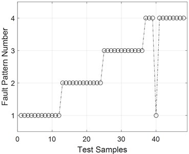
As seen in Fig. 7, the time-frequency characteristics extracted from compressed signals of different patterns can be easily separated. SVM can be used as a simple yet common method of conducting fault diagnosis. The results are shown in Fig. 8, and the accuracy of the fault diagnosis method used is determined to be 93.75 %.

Fig. 8Fault diagnosis results based on the compressed signal

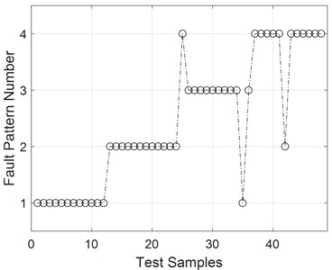
Fig. 9Fault diagnosis results based on the original signal

In contrast with the original signal, the original signal is also used to conduct fault diagnosis based on the EMD and SVM methods. Through the same process, the results of this fault diagnosis method are shown in Fig. 9, and the accuracy of the fault diagnosis method used in this case is 97.92 %. Table 3 shows the differences in diagnostic accuracy between reconstruction and the original signal.

From Table 3, it can be observed that the fault diagnosis based on the compressed signal is only lower than the fault diagnosis based on the original signal in the ball defect diagnostic. This may be due to arbitrary feature dimensionality reduction and a simple classification algorithm.

We achieved better results when we utilize regular dimensionality reduction approaches, like Kernel Principal Component Analysis (KPCA), and more sophisticated classification algorithms, such Radial Basis Function Networks (RBF), as demonstrated in Table 4.

Table 3Detail diagnosis accuracies

Signal	Normal	Inner race defect	Ball defect	Outer race defect
Original signal	100 %	100 %	100 %	91.67 %
Compressed signal	100 %	100 %	83.33 %	91.67 %

Table 4Detail diagnosis accuracies

Signal	Normal	Inner race defect	Ball defect	Outer race defect
Original signal	100 %	100 %	100 %	91.67 %
Compressed signal	100 %	100 %	83.33 %	91.67 %
Compressed signal with KPCA and RBF	100 %	100 %	100 %	100 %

Only for demonstrating that the compressed signal could preserve the time-series information and characteristic of the original signal, we employed this simple technique.

4. Conclusions

In comparison with previous compression methods that use a sample-then-compress framework, the compression method based on the Compressive Sensing theory can effectively collect and compress raw data simultaneously. In this paper, a hybrid measurement matrix is designed to compress the original signal and allow the compression signal to reserve the time-series information of the original signal. The experimental results show that the compression signal can be used for fault diagnosis based on conventional methods. The trade-off of computational complexity for remote fault diagnosis and fault diagnostic accuracy has been determined to make an impact.

References

C. K. Jha and M. H. Kolekar, “Electrocardiogram data compression techniques for cardiac healthcare systems: a methodological review,” IRBM, Jun. 2021, https://doi.org/10.1016/j.irbm.2021.06.007

Publisher
B. Hejrati, A. Fathi, and F. Abdali-Mohammadi, “A new near-lossless EEG compression method using ANN-based reconstruction technique,” Computers in Biology and Medicine, Vol. 87, pp. 87–94, Aug. 2017, https://doi.org/10.1016/j.compbiomed.2017.05.024

Publisher
S. Umamaheswari and V. Srinivasaraghavan, “Lossless medical image compression algorithm using tetrolet transformation,” Journal of Ambient Intelligence and Humanized Computing, Vol. 12, No. 3, pp. 4127–4135, Mar. 2021, https://doi.org/10.1007/s12652-020-01792-8

Publisher
G. Othman and D. Q. Zeebaree, “The applications of discrete wavelet transform in image processing: A review,” Journal of Soft Computing and Data Mining, Vol. 1, No. 2, pp. 31–43, 2020, https://doi.org/10.30880/jscdm.2020.01.02.004

Publisher
H. Kasban and S. Nassar, “An efficient approach for forgery detection in digital images using Hilbert-Huang transform,” Applied Soft Computing, Vol. 97, p. 106728, Dec. 2020, https://doi.org/10.1016/j.asoc.2020.106728

Publisher
U. Jayasankar, V. Thirumal, and D. Ponnurangam, “A survey on data compression techniques: From the perspective of data quality, coding schemes, data type and applications,” Journal of King Saud University – Computer and Information Sciences, Vol. 33, No. 2, pp. 119–140, Feb. 2021, https://doi.org/10.1016/j.jksuci.2018.05.006

Publisher
X. Tian, “Multiscale sparse dictionary learning with rate constraint for seismic data compression,” IEEE Access, Vol. 7, pp. 86651–86663, 2019, https://doi.org/10.1109/access.2019.2925535

Publisher
K. Xu, Learning in Compressed Domains. Arizona State University, 2021.

Search CrossRef
E. J. Candès, Proceedings of the International Congress of Mathematicians. Zuerich, Switzerland: European Mathematical Society Publishing House, 2007, pp. 1433–1452, https://doi.org/10.4171/022

Publisher
E. J. Candès, J. K. Romberg, and T. Tao, “Stable signal recovery from incomplete and inaccurate measurements,” Communications on Pure and Applied Mathematics, Vol. 59, No. 8, pp. 1207–1223, Aug. 2006, https://doi.org/10.1002/cpa.20124

Publisher
A. Mousavi and R. G. Baraniuk, “Learning to invert: Signal recovery via deep convolutional networks,” in 2017 IEEE International Conference on Acoustics, Speech and Signal Processing (ICASSP), pp. 2272–2276, Mar. 2017, https://doi.org/10.1109/icassp.2017.7952561

Publisher
W. Shi, F. Jiang, S. Liu, and D. Zhao, “Image compressed sensing using convolutional neural network,” IEEE Transactions on Image Processing, Vol. 29, pp. 375–388, 2020, https://doi.org/10.1109/tip.2019.2928136

Publisher
M. Haile and A. Ghoshal, “Application of compressed sensing in full-field structural health monitoring,” SPIE Smart Structures and Materials + Nondestructive Evaluation and Health Monitoring, p. 83461, Apr. 2012, https://doi.org/10.1117/12.915429

Publisher
J. Yu, X. Liu, and T. Cui, “Application research of compressed sensing in wireless sensor monitoring networks on coal mine,” ICIC express letters. Part B, Applications: an International Journal of Research and Surveys, Vol. 6, No. 6, pp. 1653–1659, 2015.

Search CrossRef
Z. Duan and J. Kang, “Compressed sensing techniques for arbitrary frequency-sparse signals in structural health monitoring,” SPIE Smart Structures and Materials + Nondestructive Evaluation and Health Monitoring, p. 90612, Mar. 2014, https://doi.org/10.1117/12.2048276

Publisher

Cited by

Adaptive Band Extraction Based on Low Rank Approximated Nonnegative Tucker Decomposition for Anti-Friction Bearing Faults Diagnosis Using Measured Vibration Data

Haobin Wen | Long Zhang | Jyoti K. Sinha

(2022)

A Sparse Recovery Algorithm Based on Arithmetic Optimization

Qingfeng Zhang | Dong Hu | Chao Tang | Jufang Xie

(2022)

About this article

Received

15 May 2021

Accepted

19 October 2021

Published

26 November 2021

SUBJECTS

Fault diagnosis based on vibration signal analysis

DOI

https://doi.org/10.21595/jve.2021.22061

Keywords

rolling bearing

remote fault diagnosis

compressive sensing

data compression

This is an open access article distributed under the Creative Commons Attribution License, which permits unrestricted use, distribution, and reproduction in any medium, provided the original work is properly cited.

Previous article in issue Previous Next article in issue Next

Research article

2024 01 21

Rolling bearing fault diagnosis based on variational mode decomposition and weighted multidimensional feature entropy fusion

Na Lei, Feihu Huang, Chunhui Li

Research article

2023 10 09

Extraction and diagnosis of rolling bearing fault signals based on improved wavelet transform

Zhiqing Cheng

Research article

2023 08 01

Rolling bearing fault diagnosis method based on ELMD hybrid feature extraction and wavelet neural network

Hengxin Yue, Xihui Chen, Xinhui Shi, Wei Lou

Research article

2020 11 24

Fault diagnosis of bearing vibration signals based on a reconstruction algorithm with multiple side Information and CEEMDAN method

Bo Wu, Yangde Gao, Na Ma, Theerasak Chanwimalueang, Xiaobing Yuan, Jianpo Liu

Z. Chen, “Rolling bearing fault diagnosis with compressed signals based on hybrid compressive sensing,” Journal of Vibroengineering, Vol. 24, No. 1, pp. 18–29, Nov. 2021, https://doi.org/10.21595/jve.2021.22061

Copy Extrica

Copied to clipboard!

TY  - JOUR
DO  - 10.21595/jve.2021.22061
UR  - https://doi.org/10.21595/jve.2021.22061
TI  - Rolling bearing fault diagnosis with compressed signals based on hybrid compressive sensing
T2  - Journal of Vibroengineering
AU  - Chen, Zihan
PY  - 2021
DA  - 2021/11/26
PB  - JVE International Ltd.
SP  - 18-29
IS  - 1
VL  - 24
SN  - 1392-8716
SN  - 2538-8460
ER  - 

Copy Ris

Copied to clipboard!

@article{Chen_2021,
	doi = {10.21595/jve.2021.22061},
	url = {https://doi.org/10.21595/jve.2021.22061},
	year = 2021,
	month = {nov},
	publisher = {{JVE} International Ltd.},
	volume = {24},
	number = {1},
	pages = {18--29},
	author = {Zihan Chen},
	title = {Rolling bearing fault diagnosis with compressed signals based on hybrid compressive sensing},
	journal = {Journal of Vibroengineering}
}

Copy Bibtex

Copied to clipboard!

[1]Z. Chen, “Rolling bearing fault diagnosis with compressed signals based on hybrid compressive sensing,” Journal of Vibroengineering, vol. 24, no. 1, pp. 18–29, Nov. 2021, doi: 10.21595/jve.2021.22061.

Copy IEEE

Copied to clipboard!

Chen, Zihan. “Rolling Bearing Fault Diagnosis with Compressed Signals Based on Hybrid Compressive Sensing.” Journal of Vibroengineering 24, no. 1 (November 26, 2021): 18–29. https://doi.org/10.21595/jve.2021.22061.

Copy Chicago

Copied to clipboard!

Rolling bearing fault diagnosis with compressed signals based on hybrid compressive sensing

Abstract

1. Introduction

2. Methodology

2.1. A brief introduction of the compressive sensing theory

2.2. Hybrid compressive sampling

2.3. Compressive feature extraction and fault classification

3. Experimental results

3.1. Comparison of the original signal and the reconstructed signal

3.2. Fault diagnosis measurement based on the compressed signal

4. Conclusions

References

Cited by

About this article

Related Articles