Abstract
Since bearing fault signal in complex running status is usually characterized as nonlinear and non-stationary, it is difficult to extract accurate affluent features and achieve effective fault identification via conventional signal processing tools. In this article, a rolling bearing fault diagnosis technique based on variational mode decomposition and weighted multidimensional feature entropy fusion is proposed to address this issue, which is mainly composed of three procedures. First, the original signal undergoes the variational model decomposition. Next, the signal features are extracted by weighted multidimensional feature entropy as the input of the diagnosis model. Finally, the classification is performed by a convolutional neural network. The method is applied in simulation and experimental analysis. The experimental results show that the proposed method, which demonstrates strong immunity to noise and robustness, can more effectively and adaptively extract the fault features of rolling bearings and achieve the goal of identifying the rolling bearing fault category and damage degree under variable operating conditions. Meanwhile, this approach exhibits superior accuracy and identification performance to some similar entropy-based hybrid approaches referred to in this article, with a promising prospect in industrial application.
Highlights
- Flowchart of WMFE algorithm
- Flowchart of rolling bearing fault diagnosis method
- Auracy of CNN traccining process by different methods
- Visualization feature distribution map using T-SNE
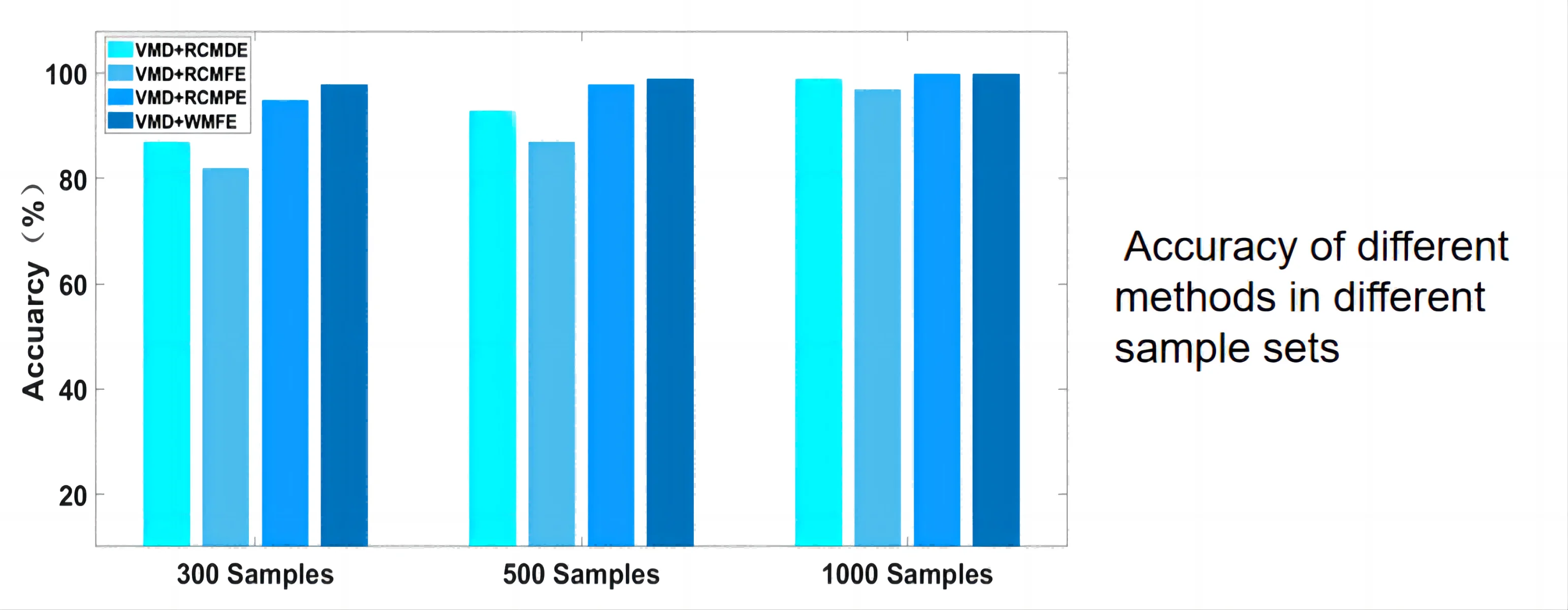
- Accuracy of different methods in different sample sets
1. Introduction
Rotating machinery, as a power equipment, has been widely used in a variety of production and processing industries. Rolling bearings are the key components of rotating machinery for power transmission, and their operating conditions directly concern the performance state of mechanical equipment [1]. Due to the harsh working environment and frequent full load operation, rolling bearings are quite easy to wear out until some fault comes about. Such a fault, once occurring, is likely to cause a series of consequences to the enterprise such as production equipment shutdown, economic loss, and personnel casualties. Therefore, monitoring the condition of rolling bearings and performing regular detection and troubleshooting are of vital significance to maintaining safe operation of the equipment. The rolling bearing fault vibration signal has a distinctive nonlinear non-stationary characteristics and contains rich and complex noise components, which makes it even difficult to extract its fault features [2].
At present, rolling bearing signal analysis methods mainly include time domain analysis, frequency domain analysis, time-frequency analysis, nonlinear analysis, graph theory, and so on. Among them, the time-frequency analysis method and the nonlinear analysis method are most commonly used. The traditional Fourier Transform (FT), a full-fledged mathematical theory with clear physical significance, has become an important tool for signal processing [3]. However, when analyzing a non-stationary signal, it is impossible to capture the time from the signal’s time series that corresponds to a particular frequency. The Short Time Fourier Transform (STFT) achieves localized analysis in the time and frequency domains by dividing the non-stationary signal into a finite number of stationary time segments via the idea of sliding windowing [4]. However, the time and frequency resolutions of the STFT method are subject to the uncertainty principle and cannot be optimized simultaneously. In addition, due to its segmentation and windowing operation, this method also has a disadvantage that the window type and size are difficult to determine. The Wavelet Transform (WT) overcomes the shortcomings of STFT owing to its fixed time-frequency resolution and is therefore widely used in rolling bearing fault diagnosis [5]. However, WT has the problems of wavelet base, fixed basis function, constant multi-resolution, and so on, which are difficult to approach. Empirical Mode Decomposition (EMD) [6] does not require setting the basis function in advance, and the signal is recursively decomposed into a series of Intrinsic Mode Function (IMF) according to the time scale. However, its theory is incomplete, lacking in essential support of a rigorous mathematical basis; there are also shortcomings due to the existence of EMD mode mixing, over-envelope, under-envelope, and so on. Therefore, Ensemble Empirical Mode Decomposition (EEMD), an improved method based on EMD is proposed to suppress the mode mixing phenomenon by introducing Gaussian white noise, and by this method the literature [7] has successfully separated the signals with distinct modes corresponding to load variations and fault effects. However, EEMD is compute-intensive, and the residual noise may cause signal reconstruction error, thereby affecting the effectiveness of feature extraction. In 2005, a new adaptive decomposition algorithm called Local Mean Decomposition (LMD) was proposed by Smith to decompose the signal into multiple PF components based on pure FM and envelope signals according to the signal’s self-characteristics without losing signal contents [8]. However, LMD still has many shortcomings, such as the defect of end effect, and the problems of riding wave processing and noise sensitivity. In 2014, Dragomiretskiy [9] proposed Variational Mode Decomposition (VMD), a new time-frequency signal analysis method based on a completely non-recursive idea, to decompose a complex signal into a series of Amplitude-Modulated-Frequency-Modulated (AM-FM) signals without high computation complexity. The adaptive decomposition of the original signal is implemented by using a non-recursive variational mode decomposition model, which is built on a solid mathematical foundation and free of the defects of EMD and LMD such as mode mixing and end effect. A novel approach has been put forward that combines particle swarm optimization kernel fuzzy C‐means (PSO‐KFCM) and VMD [10]. The conclusions drawn from the experiment show that the method can achieve good results in bearing fault diagnosis. When the rolling bearing is abnormal, the energy structure of its vibration signal will vary by the type and degree of bearing fault, so will the position of the main frequency components of the vibration signal in the frequency domain. The VMD method is used to decompose the vibration signal orthogonally in a non-redundant way, and the decomposed signal can reflect the distribution characteristics of the original signal in different frequency bands. The signal decomposed by VMD can reflect the distribution characteristics of the original signal in different frequency bands, which is essentially an enhanced representation for the original signal.
Major nonlinear analysis methods include the high-rank matrix, correlation dimension, probability density function parameters, and various types of entropy, and so on. Pincus [11] proposed Approximate Entropy (ApEn) by comparing the different findings before and after adding a white noise to a single sinusoidal signal. ApEn is an indicator of the complexity of time series with a non-negative number, and the larger the ApEn, the less regular the time series. However, due to the self-similarity drawback, the concept of ApEn is rarely applied in the machine fault diagnosis. In view of the self-similarity drawback of ApEn, Richman and Moorman [12] introduced the concept of sample entropy (SampEn) in 2000. However, what either SampEn or ApEn measured were the irregularity and self-similarity of time series on a single scale. In 2002, Costa et al. [13] introduced the enhanced concept of multi-scale entropy (MSE) to estimate the irregularity and self-similarity of time series on distinct scales and successfully characterized biological and physiological signals. Zhang et al. [14] first introduced MSE into bearing fault diagnosis and demonstrated that MSE can characterize the nonlinearity and complexity of bearing vibration signals, as well as the interaction and coupling effects between machine components, more effectively than the traditional single-scale entropy. Composite Multi-scale Entropy (CMSE) was proposed on the basis of MSE, and it can solve the problems of inaccurate and larger fluctuations of entropy values existing in MSE, but not the problem of undefined entropy induced by too short sample time series [15], Refined Composite Multi-scale Entropy (RCMSE) proposed by Wu et al. is a new algorithm [16] to improve the accuracy of entropy estimation and reduce the probability of inducing undefined entropy. CHEN et al. [17] proposed Fuzzy Entropy (FE) on the basis of sample entropy, using an exponential function instead of the step function such that the entropy value has better continuity. However, the affiliation function used by Chen et al. in FE lacks physical significance and statistical significance; Combining the concept of FE, Zheng Jinde et al. [18] proposed Multi-scale Fuzzy Entropy (MFE) and applied it to the fault diagnosis of rolling bearings, showing that MFE is an effective method to measure the complexity of time series. Compared with single-scale entropy, it can reflect the holistic dynamics and reveal its evolutionary characteristics in detail. However, its multi-scale coarse-grained process may lead to fluctuations in entropy on larger scales and to the phenomenon of end “flying wing”. This is why Zheng et al. [19] proposed Composite Multi-scale Fuzzy Entropy (CMFE) to improve the stability and continuity of the entropy curve, though there remains the problem of undefined local entropy. The literature [20] applied Refined Composite Multi-scale Fuzzy Entropy (RCMFE) to the field of fault diagnosis and verified that RCMFE can accurately extract the information of vibration signal fault characteristics with excellent entropy stability. Permutation Entropy (PE) [21] is another method that can reflect the nonlinear dynamic characteristics of the vibration signal, and which is applied in the field of rolling bearing fault diagnosis with good diagnostic results. Zheng Jinde et al. [22] extracted the PE of the components by decomposing the vibration signal for rolling bearing fault diagnosis. Multi-scale Permutation Entropy (MPE) is defined as the PE with multi-scale factors, which enables effective access to the vibration information of vibration signals with multi-scale factors and effective characterization of random mutative behaviors of the time series, as compared with single-scale permutation entropy [23]. However, in the MPE algorithm, as the scale factor increases, the coarse-grained process tends to shorten the time series, inevitably leading to a lack of characteristic information of the vibration signal on larger scales. For this reason, Refined Composite Multi-scale Permutation Entropy (RCMPE) was also proposed in the literature [24], and it is much less dependent than MPE on signal length. In this sense, RCMPE is more reliable than MPE. Despite the wide application of ApEn, SampEn, and PE, they each have shortcomings: ApEn cannot make a clear distinction between signals with low complexity; SampEn is not fast enough for long signals and is susceptible to mutated signals; PE fails to allow for the difference between amplitude averages and amplitude values. Rostaghi et al. [25] proposed a new irregular indicator of Dispersion Entropy (DE), which has overcome the limitations of PE and SE mentioned above while allowing for the relationship between amplitudes, with lower susceptibility to mutated signals and higher stability, and faster computation speed. In order to comprehensively and systematically reflect the uncertainty and complexity of time series, Azami et al. extended the DE at multi-scale into Multi-scale Dispersion Entropy (MDE), which reflects the complexity of time series at multiple time scales. MDE has not only addressed the problem of low stability of multi-scale coarse granulation, but also achieved a great improvement in accuracy. On the basis of DE, this paper proposes Composite Multi-scale Dispersion Entropy (CMDE), which demonstrates higher stability than traditional coarse-grained multi-scale procedures, to solve the problem of incomplete extraction of signal complexity features by single-scale DE. This technique also has some other advantages in computational error and feature extraction. The literature [26] also proposed Refined Composite Multi-scale Dispersion Entropy (RCMDE), which is applied in feature extraction from biological signals, and the entropy outperform several other types of multi-scale entropies in terms of computational error and feature extraction. Over the past few years, a few researchers have illustrated the advantages of RCMDE, RCMFE and RCMPE over the conventional methods. A detailed comparison between most of the above-mentioned entropy [27]. Minhas et al. proposed a new method for bearing fault diagnosis and identification based on Complementary Ensemble Empirical Mode Decomposition (CEEMD) and weighted multi-scale entropy method [28]. The information represented by the quantitative single entropy index is limited, only capable to reflect the single characteristic information of time series; the analytic effect has certain limitations, such as not being capable to fully reflect the fault information of rolling bearing signal, and the inferior adaptability when a single entropy is used to represent the signal characteristic information. Therefore, it is necessary to take advantage of the complementary nature of the differences between different entropies to build a more comprehensive representation for the signal information of the high-dimensional feature set. To integrate the RCMDE, RCMFE and RCMPE methods with more effectiveness to reflect the characteristics of vibration signals more comprehensively, it is imperative to develop a robust technique which comprises critical and influential weighted parameters. The objective of including such parameters is to offset the entropy output values appropriately without actually interfering in the intrinsic characteristics of any particular entropy method. To make objective evaluation of the contribution of each entropy to signal feature extraction, this paper proposes a Weighted Multidimensional Feature Entropy (WMFE) method based on linear weighted single entropy, in which the weight of each entropy is calculated using the Standard Deviation Method (SDM) [29]. WMFE takes advantage of the complementary nature of the differences between different feature entropies to construct a more comprehensive high-dimensional feature vector set to represent fault type information and reflect the characteristics of the signal more comprehensively.
Convolutional Neural Network (CNN) is a supervised deep learning algorithm developed in recent years [30], which has been applied in the field of fault diagnosis by scholars for its powerful capability in automatic feature extraction. In the literature [31] CNN was used to achieve bearing fault diagnosis and lubrication performance degradation in rotating machinery. Zhang et al. [32] proposed a CNN model based on the adaptive batch normalization (AdaBN) algorithm, which enabled adaptive feature extraction for bearing fault diagnosis under variable working conditions. CNN is capable of self-adaptively extracting multidimensional data abstract features; after being fused with a fully-connected network, it can achieve the result of automatic feature extraction oriented to the diagnostic target, namely the feature extraction from the effect to the cause, and avoid the uncertainty of manual feature screening.
Synthesize the advantages of the above methods, a rolling bearing fault diagnosis method based on VMD and WMFE fusion is proposed in this paper. The procedure starts with decomposing the vibration signals of different fault categories of rolling bearings under variable working conditions by VMD; next, WMFE is extracted from the decomposed IMF components, which are then integrated into a high-dimensional data grid in matrix form and input into CNN for a judgment on the fault categories of rolling bearings. This way, accurate diagnosis of fault categories and damage severity of rolling bearings are achieved under variable working conditions.
2. Algorithm introduction
2.1. VMD
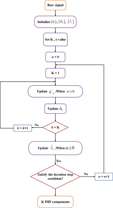
The VMD algorithm is a non-recursive adaptive signal decomposition method, with its decomposition process shown in 0. The signal is decomposed into a number of AM-FM IMFs, and the process can be expressed as:
where is the current time; the phase is a non-decreasing function of ; is the th decomopsed IMF component; is the instantaneous amplitude and is a non-negative envelope function; is the number of decomposition.
The process of constructing the variational mode is as follows:
(1) The analytic signal of IMF is obtained by Hilbert Transform, and thus the one-sided spectrum of the signal is obtained.
(2) The exponential term is used to adjust the center frequency of each IMF and transform each IMF frequency to the fundamental frequency band.
(3) The bandwidth of each IMF component is calculated using the Gaussian smoothing demodulated signal. The constructed variational mode is:
where: is the input signal; is the unit impulse function; is the center frequency; is the convolution operation.
An extended Lagrangian function given by the following expression is introduced to solve the optimal solution of the variational mode:
where: is the penalty factor; is the Lagrange multiplier.
The Alternate Direction Method of Multipliers (ADMM) is used to update , and to obtain the saddle point of the Lagrangian function, hence the optimal solution of Eq. (3). The Fourier Transform is used to update Eq. (3) from the time domain to the frequency domain:
where: is the fidelity factor; is the number of iterations; is the frequency; denotes the Fourier Transform.
Repeat Eq. (4) through Eq. (6) until satisfying the following iteration stopping condition where the update can come to a stop:
where: is the discriminatory accuracy which takes 10-6.
By the time the iteration stops, the frequency-domain characteristics of the signal have been decomposed adaptively, and the modulated signal has been transformed into the time-domain IMF component using the inverse Fourier Transform.
Fig. 1Flowchart of VMD algorithm
2.2. WMFE
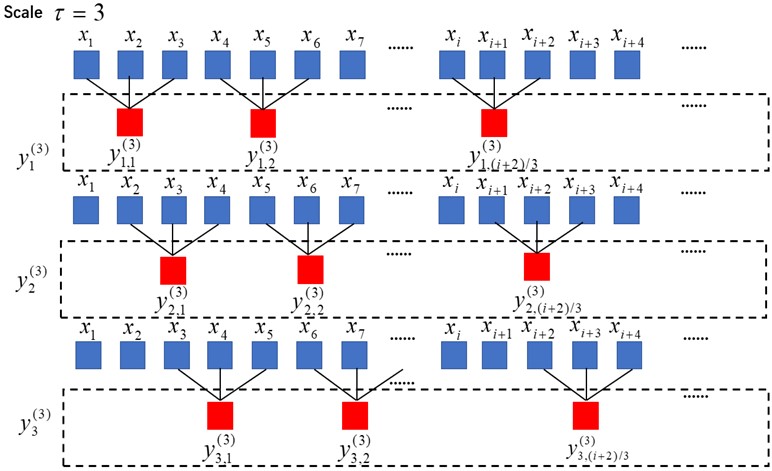
Based on the RCMSE, three entropy methods, RCMDE, RCMFE and RCMPE, have been established in the fields of biomedical engineering and mechanical fault diagnosis. All these methods have the same coarse-grained process with a scale factor of 3, as shown in 0, Suppose a time series , where is the total length of the signal. Given a scale factor, , the th coarse-grained sequence of is given by:
The steps to calculate the RCMDE are described as follows.
(1) Let 1. The DE of the time series is calculated as follows.
a) Map the coarse-grained time series into the class ( is a positive integer). This process needs to be implemented in two substeps: First, map the coarse-grained series onto the interval (0, 1) by Eq. (9) for the normal cumulative distribution function (NCDF):
where: and denote the mean and standard deviation of , respectively.
Next, map to class in the form of by linear transformation, where is the rounding operation.
b) Given the embedding dimension and the time delay reconstruct the time series , where .
c) Assuming that each time series corresponds to a dispersion pattern, let , , …, , then corresponds to a dispersion pattern , where the largest dispersion pattern does not exceed .
d) The probability of each dispersion pattern is calculated as follows:
where the term indicates the number of corresponding to the dispersion pattern.
e) Therefore, DE can be calculated as:
(2) Repeat step (1) for to obtain DE at multi-scale. Thus, the RCMDE expression is given by:
where .
The steps to calculate the RCMFE are described as follows.
(1) Let 1. The FE calculation substeps for the time series are as follows.
a) Given the embedding dimension and time delay , reconstruct the coarse-grained time series into the following time series , where , .
b) The maximum absolute distance between and is calculated using where, , .
c) Defining the fuzzy weight as and the similarity tolerance as , the similarity between and is calculated by the fuzzy relationship function .
d) Where by:
e) FE is obtained by the natural logarithm ratio of the continuous function in substep d):
(2) Repeat step (1) for at multi-scale to obtain FE. Thus, the RCMFE expression is given by:
where , .
Fig. 2Coarse-grained process of time series
The steps to calculate the RCMPE are described as follows.
(1) Let 1. The PE of the time series is calculated as follows.
a) Given the embedding dimension and the time delay , reconstruct the coarse-grained time series into the time series , which is arranged in ascending order according to the numerical value of the elements. There are possible permutations for the patterns, and for each permutation of pattern –, the relative frequency is obtained as follows:
b) PE is calculated as follows:
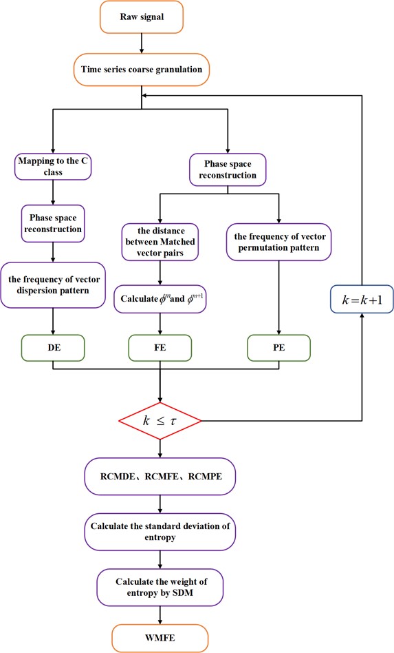
Fig. 3Flowchart of WMFE algorithm
(2) Repeat step (1) for to obtain PE at multi-scale. Thus, the RCMPE expression is given by:
where .
The steps to calculate the WMFE are described as follows, with the flowchart of the algorithm shown in 0.
(1) The formula for calculating the weights using the standard deviation method is given by:
where, is RCMDE, RCMFE or RCMPE; is the variance of the th entropy.
(2) The variance formula for calculating entropy is given by:
where, is the entropy at the th scale; is the mean value of entropies.
Therefore, the WMFE expression is given by:
2.3. Algorithm parameter setting
2.3.1. Setting of parameter of VMD
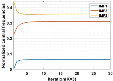
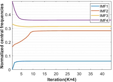
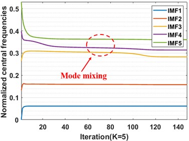
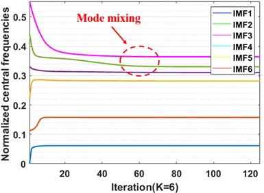
In the process of VMD decomposition of vibration signal samples, the choice of the preset modal number and penalty factor is decisive to whether the VMD can accurately decompose the vibration signal; too small a value of may cause mode aliasing or mode loss, while too great a value of may lead to over-decomposition. In this paper, we determine whether over-decomposition occurs – and then the value of the preset mode number – by observing the change of the center frequency of each mode component after VMD decomposition [33]. Taking the inner race fault with a fault size of 0.021 inches as an example, the penalty factor is set to 2000. 0 shows the center frequency curves when is equal to 3, 4, 5, and 6, respectively, in the VMD iteration process. From 0, the two curves move closer when 5 or 6, which means mode aliasing. When 4, the center frequency curve of each model component makes no difference to each other. This indicates that this is the most suitable number of VMD decomposition layers. For this reason, the parameter is set to 4 in this paper.
2.3.2. Parameter setting of RCMDE, RCMFE and RCMPE
From Eqn. (12), four parameters are needed to calculate RCMDE: number of classes , embedding dimension , time delay , and scale factor . It is generally recommended that the value of be set to an integer between 4 and 8. For the embedding dimension , although a larger value of m can reconstruct the dynamic process in more detail, an overly large value of will require many data points, while the length of most data in the real world is always finite; on the other hand, too small a value of may result in insufficient information. In this paper, is kept 2. To prevent information loss, the time delay is usually set as 1. Considering that too large a value ofincreases the computational quantity, while too small a value offalls short of extracting enough information for preventing the feature vector from growing too large and for ensuring a balance between performance and computational efficiency [34], in this paper the scale factor is kept 20, i.e., the RCMDE are extracted by a scale factor of 20 for data samples. In addition, the embedding dimension of RCMFE is the same as that of RCMDE, which is kept 2. And determines the width and gradient of the fuzzy affiliation function boundary. Too narrow a fuzzy affiliation function will make the final estimation of statistical properties inaccurate and sensitive to noise, while too wide a fuzzy affiliation function may lead to a loss of detailed information, so the value of is kept 2. The similarity tolerance determines the similarity of matching. The larger the value is, the more data information will be lost, while the smaller it is, the more sensitive it is to noise. And is generally recommended to be 0.1-0.25 times the SD (Standard Deviation) of the original data, and thus kept 0.15 SD in this paper [35]. Time delay and scale factor are the same for RCMDE. In calculating RCMPE, too large a value of makes it difficult to identify the dynamic changes in the time series, while too small a value of may impede the RCMPE from working due to the much smaller number of different states (symbols) [36]. In this paper, is kept 3, and the parameters of time delay and scale factor are the same as above.
Fig. 4Central frequency curves
2.3.3. Parameter setting of CNN
The detailed structure and parameter settings of the CNN network model are shown in 0. Firstly, a high-dimensional feature vector matrix composed of WMFE is input to the first convolutional layer Conv_1 network with 32 convolutional kernels and the activation function is Relu, which is self-normalized to the data. Subsequently, the maximum pooling is connected, and the output features are processed by taking the maximum value and discarding the remaining spatial features to achieve the purpose of feature dimensionality reduction. Then it is fed into the second convolutional layer, Conv_2 network, with 32 convolutional kernels, using the Relu activation function, followed by the maximum pooling operation. The last layer is the fully connected layer, and the Softmax activation function is applied to classify the output results into 10 types of faults. The hyperparameters are set as follow, the learning rate is 0.001, the number of small batches is 10, the number of iterations is 10, and the loss function is the cross-entropy.
Table 1CNN convolutional neural network parameter design
Network layer type | Convolutional kernel size/steps | Number of convolutional kernels | Input size | Output size | Activation function |
Input layer | 10×4×20×3 | 10×4×20×3 | Relu | ||
Conv_1 | 2×2/1 | 32 | 10×4×20×3 | 10×4×20×32 | Relu |
Batch normalization | 10×4×20×32 | 10×4×20×32 | |||
Max pooling_1 | 2×2/1 | 10×4×20×32 | 10×2×10×32 | ||
Conv_2 | 2×2/1 | 32 | 10×2×10×32 | 10×2×10×32 | Relu |
Max pooling_2 | 2×2/1 | 10×2×10×32 | 10×1×5×32 | ||
Flatten | 10×1×5×32 | 10×160 | |||
Dense_1 | 10×160 | 10×16 | Relu | ||
Dense_2 | 10×16 | 10×10 | Softmax |
2.4. Rolling bearing fault diagnosis based on VMD and WMFE Fusion
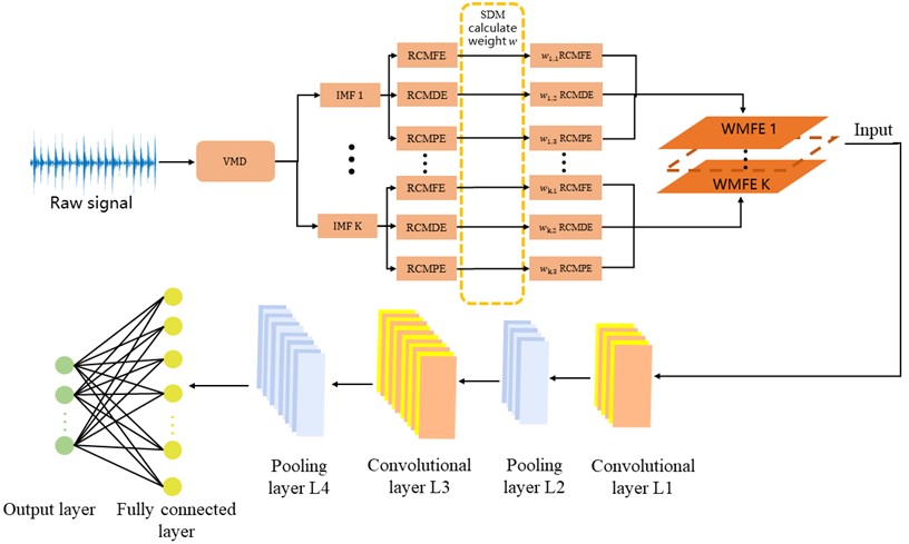
Based on the good robustness of VMD, end effect suppression, fewer model pseudo-components, and the advantages of WMFE being capable to extract multidimensional signal feature vectors adaptively, the fault diagnosis process is designed as shown in 0 The rolling bearing fault diagnosis based on VMD and WMFE fusion includes three major parts: VMD of the original signal, extraction of WMFE characteristic information, and CNN neural network classification. The procedure starts with decomposing the rolling bearing vibration signal under variable working conditions by VMD; next, RCMDE, RCMFE and RCMPE feature vectors are extracted from IMFs and weights are obtained using SDM, which are then assembled into WMFE data grid in matrix form and input into CNN. After the convolution layer of the multi-scale convolution kernel and the maximum pooling and dimension reduction of the multi-scale features in high dimension, the final input fully connected layer for classification by the Softmax activation function.
Fig. 5Flowchart of rolling bearing fault diagnosis method
3. Analysis of simulation signals
3.1. Construction of a data set for rolling bearing simulation signals
Based on the structural characteristics of rolling bearings, a component of the bearing, when damaged in the bearing operation process where other components collide with each other, excites a shock signal in the form of high-frequency damped oscillation and an inherent vibration at high frequency. The vibration signal simulation model for rolling bearing fault diagnosis is expressed as follows [37]:
where: is the time fluctuation of the th shock interval with respect to the shock period ; is an exponentially decaying sinusoidal signal vibrating at the intrinsic frequency ; is the system damping ratio; is the amplitude modulated signal; and are random numbers; is a random signal with mean 0; is the modulation frequency, which depends on the fault type. In case of outer race fault, is 0; in case of inner race fault, is the axis rotation frequency; in case of ball fault, is the cage rotation frequency.
Due to the complexity of long-term high-speed working conditions and the special characteristics of their structure, rolling bearings are prone to compound faults, and multiple fault characteristics are superimposed on and interfere with each other, increasing the difficulty of feature extraction from compound faults. (outer race), (inner race), and (ball) are the vibration simulation signals for single faults of rolling bearings, whereas (outer race & inner race), (outer race & ball), and (inner race & ball) are the vibration simulation signals for compound faults of rolling bearings:
where: = 600, = 800, = 600, = 3000 Hz, = 5000 Hz, = 2000 Hz, = 25 Hz, = 5 Hz, = 1/50, = 1/90, =1/40, sampling frequency = 1.6 kHz.
Figure 6 shows the temporal waveforms and FFT spectra of the 6 simulation signals to which the Gaussian white noise has been added with a signal-to-noise ratio (SNR) of –4 dB. The SNR equation is given as follows. According to in 0, it is impossible to distinguish fault types by directly observing the six temporal signals due to noise interference. Besides, from the FFT spectra in Fig. 6, the characteristic information of all other frequency bands but the resonance frequency band is quite similar, which means it is necessary to adopt an effective technique to process the information [38]:
where: is the input signal power, and is the noise power.
Gaussian white noise signals with distinct SNRs are added to , , , , , and , forming the simulation vibration signals for rolling bearing faults with SNRs ranging within [–4, 8]. The number of training sets and test samples at each ratio of these signals are 40 and 10, respectively, with sample length 5000, summing up to 1680 training set samples and 420 testing set samples. The data sets are described in Table 2.
Fig. 6Temporal waveform and FFT spectrum of 6 simulation signals (SNR = –4 dB)
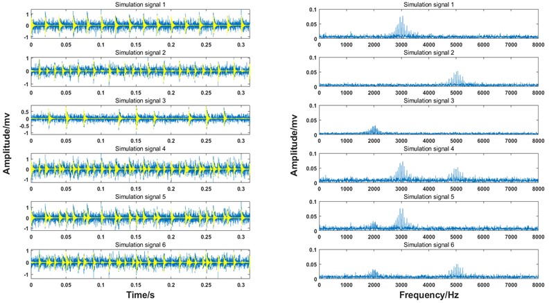
Table 2Rolling bearing simulation data set
Fault type | SNR/ dB | |||||||
–4 | –2 | 0 | 2 | 4 | 6 | 8 | ||
Simulation signals 1 | Training set | 40 | 40 | 40 | 40 | 40 | 40 | 40 |
Testing set | 10 | 10 | 10 | 10 | 10 | 10 | 10 | |
Simulation signals 2 | Training set | 40 | 40 | 40 | 40 | 40 | 40 | 40 |
Testing set | 10 | 10 | 10 | 10 | 10 | 10 | 10 | |
Simulation signals 3 | Training set | 40 | 40 | 40 | 40 | 40 | 40 | 40 |
Testing set | 10 | 10 | 10 | 10 | 10 | 10 | 10 | |
Simulation signals 4 | Training set | 40 | 40 | 40 | 40 | 40 | 40 | 40 |
Testing set | 10 | 10 | 10 | 10 | 10 | 10 | 10 | |
Simulation signals 5 | Training set | 40 | 40 | 40 | 40 | 40 | 40 | 40 |
Testing set | 10 | 10 | 10 | 10 | 10 | 10 | 10 | |
Simulation signals 6 | Training set | 40 | 40 | 40 | 40 | 40 | 40 | 40 |
Testing set | 10 | 10 | 10 | 10 | 10 | 10 | 10 | |
3.2. Comparative analysis of simulation
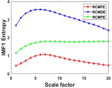
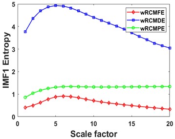
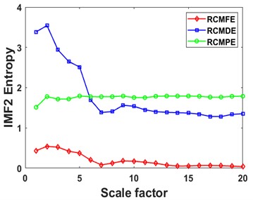
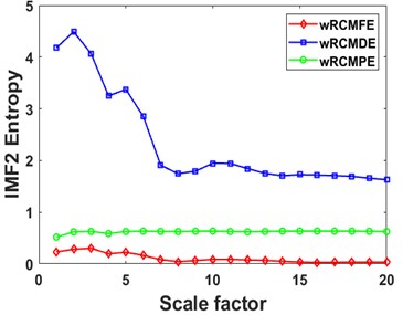
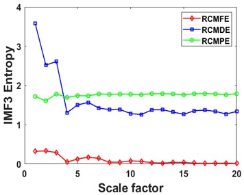
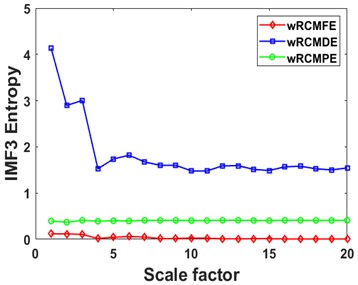
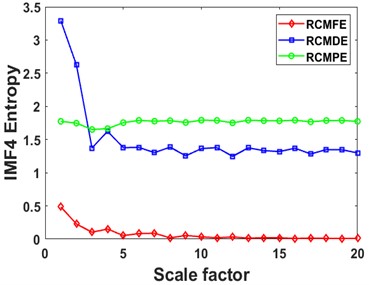
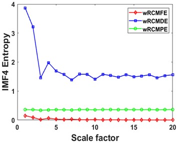
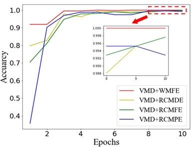
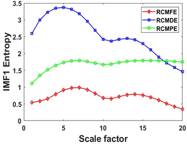
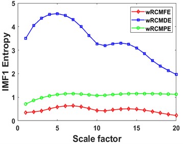
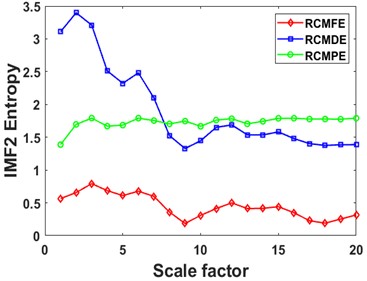
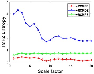
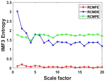
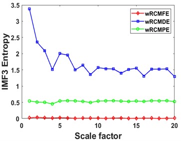
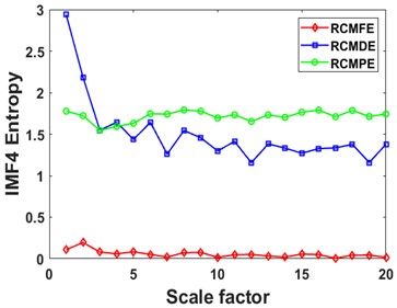
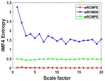
First, each rolling bearing simulation signal is decomposed by VMD into 4 IMF components. These IMFs with distinct center frequencies contain all the characteristic information of the simulation signal, as shown in Fig. 7. Then the RCMDE, RCMFE, and RCMPE of the IMFs are calculated via SDM to obtain the WMFE of the IMFs with entropy weights, as shown in Fig. 8, which correspond to the curves of different entropies of the 4 IMFs. It can be seen that the separability of the RCMDE, RCMFE, and RCMPE values of each IMF after weighting has been enhanced, which verifies that the WMFE method delivers higher accuracy than do the existing entropy methods in estimating the complexity of the signal at each scale. Compared with RCMDE, RCMFE, and RCMPE, as shown in Fig. 9, the recognition rate of the proposed WMFE method converges fast, up to 99.52 % at the third time and 100 % at the fifth time, while the recognition rates of RCMDE and RCMPE finally reach 99.29 % and 99.76 %, respectively; the effect of RCMPE is slightly worse, and its recognition rate finally reaches 99.29 %. Therefore, WMFE outperforms the other entropy methods in recognition rate, convergence speed, and noise immunity according to the simulation data.
Fig. 7The VMD of rolling ball fault simulation signal (ball fault –4 dB)
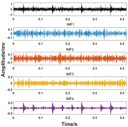
Fig. 8Curves of different entropies of 4 IMFs: a), b) IMF1, c), d) IMF2, e), f) IMF3, and g), h) IMF4
a)
b)
c)
d)
e)
f)
g)
h)
Fig. 9Accuracy of CNN training process by different methods
4. Actual signal analysis
To verify the effectiveness and accuracy of the proposed method, the experiments in this paper are conducted with rolling bearing data collected from Case Western Reserve University (CWRU)[39], which are widely used for rolling bearing fault diagnosis.
4.1. Description of dataset
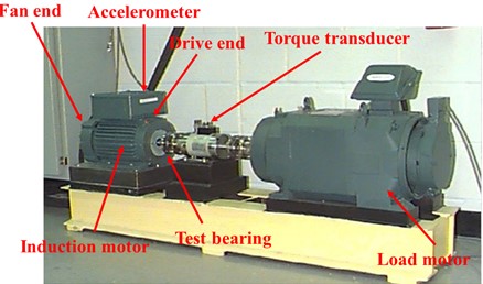
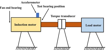
As shown in Fig. 10, the experimental platform consists of four components: a motor, a torque transducer, a power tester, and a controller. The faulty bearing under test is the drive end bearing of model SKF6205 motor. The electric spark method was used to machine single-point grooves with damage diameters of 0.007 inches, 0.014 inches, and 0.021 inches on the surfaces of the inner race, ball and outer race, respectively, to simulate the wear process of the rolling bearing in real operation. At a sampling frequency of 12 kHz in this experiment, the acceleration data sets were collected at the speed of 1772 r/min, 1750 r/min, and 1730 r/min, corresponding to the load of 1 hp, 2 hp, and 3 hp, respectively; the collected data were divided into 10 types according to the location and degree of different damages. As shown in 0, 5000 sampling points are set for each segment, and 1,000 samples are selected randomly from the 10 types and divided into the training samples and test samples at a ratio of 4:1. The data set for the experimental variable working condition is described in Table 3.
Fig. 10Experimental apparatus for bearing: a) physical diagram, b) structural sketch
a)
b)
Fig. 11Time-domain waveforms of CWRU bearing data for 10 different states
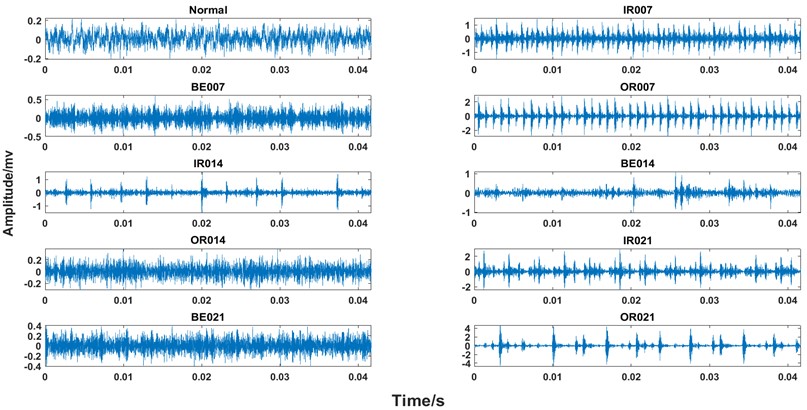
Table 3Data set of rolling bearing experimental variable working conditions
Defect size / inch | Motor load / hp | Motor speed / r⋅min-1 | Inner / label | Training set | Testing set | Ball/label | Training set | Testing set | Outer / label | Training set | Testing set |
No defect | 1 hp | 1772 | Normal/0 | 240 | 65 | ||||||
2 hp | 1750 | ||||||||||
3 hp | 1730 | ||||||||||
0.007 | 1 hp | 1772 | IR007/1 | 45 | 18 | B007/2 | 68 | 17 | OR007/3 | 59 | 15 |
2 hp | 1750 | ||||||||||
3 hp | 1730 | ||||||||||
0.014 | 1 hp | 1772 | IR014/4 | 71 | 19 | B014/5 | 66 | 18 | OR014/6 | 66 | 11 |
2 hp | 1750 | ||||||||||
3 hp | 1730 | ||||||||||
0.021 | 1 hp | 1772 | IR021/7 | 61 | 14 | B021/8 | 63 | 12 | OR021/9 | 61 | 11 |
2 hp | 1750 | ||||||||||
3 hp | 1730 |
4.2. Experimental comparative analysis
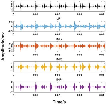
First, considering that VMD features adaptive signal decomposition, the rolling bearing vibration signal is decomposed by VMD into 4 IMF components. These IMF components with distinct center frequencies contain all the characteristic information of the rolling bearing vibration signal, as shown in Fig. 12.
Fig. 12The VMD of rolling ball fault signal(ball)
Then the RCMDE, RCMFE, and RCMPE of the IMFs are calculated via SDM to obtain the WMFE of the IMFs with entropy weights, as shown in Fig. 13, which correspond to the curves of different entropies of the 4 IMFs. It can be seen that the separability of the RCMDE, RCMFE, and RCMPE values of each IMF after weighting has been enhanced, which verifies that the WMFE method delivers higher accuracy than do the existing entropy methods in estimating the complexity of the signal at each scale. In this paper, the high-dimensional data are represented by the low-dimensional distribution of the T-SNE method. As shown in Fig. 14, the T-SNE visualizations of the WMFE, RCMDE, RCMFE, and RCMPE methods are presented for the 200 validation sets classified with the signal features extracted from them each. Evidently, the T-SNE visualization of WMFE for extracting features from rolling bearing signals has very distinctive classification features; the same categories are clustered at the same location, and the inter class distance is relatively much great; the 10 categories are independently separated from each other. In contrast, the classification results of the RCMDE, RCMFE and RCMPE methods are cluttered in the two-dimensional space and are much less effective than the WMFE method. The features extracted by the WMFE method are definitely far more sensitive than by other entropy methods, and thus the performance of WMFE is verified. This performance upgrade is owing to WMFE taking advantage of the complementary nature of the differences between different feature entropies and combining the advantages of the RCMDE, RCMFE and RCMPE methods with more effectiveness, to build a more comprehensive representation for the signal information of the high-dimensional feature set and for the characteristics of fault type information.
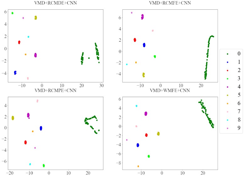
To verify the effectiveness of the method under real working conditions, the proposed method is compared with the RCMDE, RCMFE, and RCMPE methods, with the results shown in Fig. 15. The recognition rate of the WMFE method has converged to 98 % at the 3rd iterations, and stabilized to 100 % at the 4th iteration, while the maximum recognition rates of RCMFE and RCMDE are both 100 %. Nevertheless, they show unstable trends and fluctuations during the iterative process. Although RCMPE can also reach 100 % recognition rate eventually, its convergence speed is far inferior to that of the WMFE method, so WMFE significantly outperforms the other three methods. The combined VMD and WMFE methods are compared with WMFE, to find that the results of fault diagnosis by the former method are relatively satisfactory, probably because VMD decomposes and separates the vibration signal with distinct amplitude and frequency characteristics, thereby essentially enhancing the original signal. The processing results via CNN are visualized in Fig. 16. The VMD and WMFE combined feature extraction method is capable to completely separate the 10 states with the optimal intra class distance and inter class spacing compared with the previous 3 methods.
Fig. 13Curves of different entropies of 4 IMFs: a), b) IMF1, c), d) IMF2, e), f) IMF3, and g), h) IMF4
a)
b)
c)
d)
e)
f)
g)
h)
Fig. 14Visualization feature distribution map using T-SNE
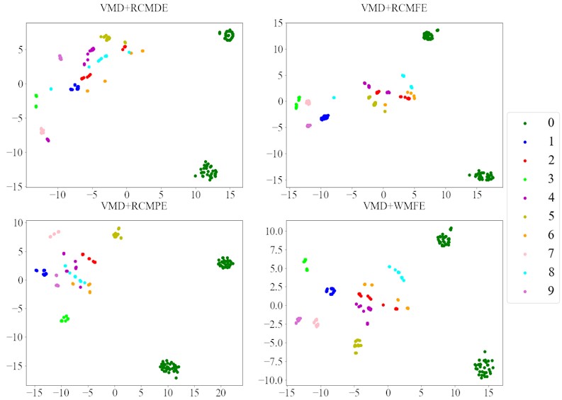
Fig. 15Accuracy of CNN training process by different methods
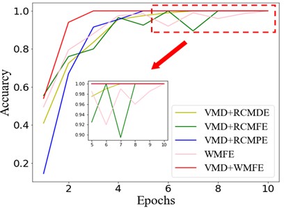
Fig. 16Visualization feature distribution map using T-SNE
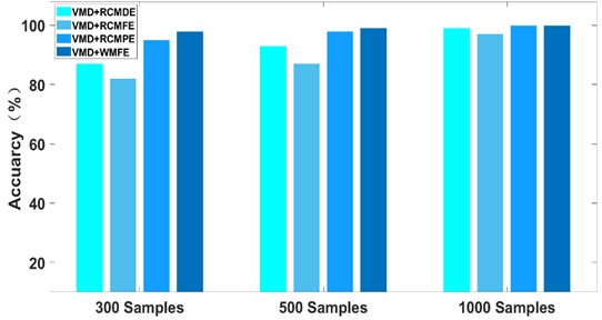
Considering that the performance of the WMFE method may differ by the size of data samples, three sets of 300, 500, and 1000 faulty samples were created for comparison experiments and divided into training sets and testing sets at a ratio of 4:1. According to the results shown in Fig. 17, the WMFE method delivers the highest accuracy among the 300, 500, and 1000 samples. In particular, for small sample sets, WMFE can extract rolling bearing signal features with higher accuracy for taking advantage of the complementary nature of the differences between different entropies to build a more comprehensive representation for the signal information of the high-dimensional feature set. Therefore, the performance and robustness of the method proposed in this paper are superior to the counterparts of RCMDE, RCMFE and RCMPE in extracting signal features.
Fig. 17Accuracy of different methods in different sample sets
5. Conclusions
In this paper, a rolling bearing fault diagnosis method based on VMD and WMFE fusion has been proposed to achieve adaptive diagnosis of different fault types and damage degrees of rolling bearings under variable working conditions. Through the simulation analysis, it has been verified that the WMFE method delivers higher accuracy than do other entropy methods in estimating the complexity of the signal at multi-scale. Also, this novel method can be used to extract the features of the signal more effectively and comprehensively enhanced feature vectors, and it outperforms RCMDE, RCMFE and RCMPE. Then, a validity analysis has been conducted by applying this method to the data of rolling bearings collected from Western Reserve University, followed by a comparative analysis with RCMDE, RCMFE and RCMPE. The experimental results show that the fault signal features extracted by the method deliver higher classification accuracy in bearing fault diagnosis irrespective of the type of bearing faults and the severity of faults. This method has also proven effective in identifying the type and location of bearing faults with higher recognition accuracy than the other 3 methods. The method has superior ability in extracting rolling bearing signal features and stronger noise immunity, self-adaptability and robustness under variable speed conditions, providing an effective way for rolling bearing fault diagnosis.
References
-
S. Adamczak, K. Stępień, and M. Wrzochal, “Comparative study of measurement systems used to evaluate vibrations of rolling bearings,” Procedia Engineering, Vol. 192, pp. 971–975, Jan. 2017, https://doi.org/10.1016/j.proeng.2017.06.167
-
Wei, Li, Xu, and Huang, “A review of early fault diagnosis approaches and their applications in rotating machinery,” Entropy, Vol. 21, No. 4, p. 409, Apr. 2019, https://doi.org/10.3390/e21040409
-
V. K. Rai and A. R. Mohanty, “Bearing fault diagnosis using FFT of intrinsic mode functions in Hilbert-Huang transform,” Mechanical Systems and Signal Processing, Vol. 21, No. 6, pp. 2607–2615, Aug. 2007, https://doi.org/10.1016/j.ymssp.2006.12.004
-
H. Tao, P. Wang, Y. Chen, V. Stojanovic, and H. Yang, “An unsupervised fault diagnosis method for rolling bearing using STFT and generative neural networks,” Journal of the Franklin Institute, Vol. 357, No. 11, pp. 7286–7307, Jul. 2020, https://doi.org/10.1016/j.jfranklin.2020.04.024
-
X. Tao et al., “Bearings fault detection using wavelet transform and generalized Gaussian density modeling,” Measurement, Vol. 155, p. 107557, Apr. 2020, https://doi.org/10.1016/j.measurement.2020.107557
-
G. Georgoulas, T. Loutas, C. D. Stylios, and V. Kostopoulos, “Bearing fault detection based on hybrid ensemble detector and empirical mode decomposition,” Mechanical Systems and Signal Processing, Vol. 41, No. 1-2, pp. 510–525, Dec. 2013, https://doi.org/10.1016/j.ymssp.2013.02.020
-
H. Mahgoun, F. Chaari, A. Felkaoui, and M. Haddar, “Early detection of gear faults in variable load and local defect size using ensemble empirical mode decomposition (EEMD),” in Applied Condition Monitoring, Cham: Springer International Publishing, 2016, pp. 13–22, https://doi.org/10.1007/978-3-319-41459-1_2
-
Y. Liu, T. Wu, J. Chen, S. Fan, X. Liu, and Y. Gong, “Research on local mean decomposition and extreme learning machine based circuit breaker fault diagnosis method,” in 2020 Asia Energy and Electrical Engineering Symposium (AEEES), May 2020, https://doi.org/10.1109/aeees48850.2020.9121481
-
K. Dragomiretskiy and D. Zosso, “Variational mode decomposition,” IEEE Transactions on Signal Processing, Vol. 62, No. 3, pp. 531–544, Feb. 2014, https://doi.org/10.1109/tsp.2013.2288675
-
Y. Chang, G. Bao, S. Cheng, T. He, and Q. Yang, “Improved VMD‐KFCM algorithm for the fault diagnosis of rolling bearing vibration signals,” IET Signal Processing, Vol. 15, No. 4, pp. 238–250, Apr. 2021, https://doi.org/10.1049/sil2.12026
-
S. M. Pincus, “Approximate entropy as a measure of system complexity.,” Proceedings of the National Academy of Sciences, Vol. 88, No. 6, pp. 2297–2301, Mar. 1991, https://doi.org/10.1073/pnas.88.6.2297
-
J. S. Richman and J. R. Moorman, “Physiological time-series analysis using approximate entropy and sample entropy,” American Journal of Physiology-Heart and Circulatory Physiology, Vol. 278, No. 6, pp. H2039–H2049, Jun. 2000, https://doi.org/10.1152/ajpheart.2000.278.6.h2039
-
M. Costa, A. L. Goldberger, and C.-K. Peng, “Multiscale entropy analysis of complex physiologic time series,” Physical Review Letters, Vol. 89, No. 6, p. 068102, Jul. 2002, https://doi.org/10.1103/physrevlett.89.068102
-
L. Zhang, G. Xiong, H. Liu, H. Zou, and W. Guo, “Bearing fault diagnosis using multi-scale entropy and adaptive neuro-fuzzy inference,” Expert Systems with Applications, Vol. 37, No. 8, pp. 6077–6085, Aug. 2010, https://doi.org/10.1016/j.eswa.2010.02.118
-
S.-D. Wu, C.-W. Wu, S.-G. Lin, C.-C. Wang, and K.-Y. Lee, “Time series analysis using composite multiscale entropy,” Entropy, Vol. 15, No. 3, pp. 1069–1084, Mar. 2013, https://doi.org/10.3390/e15031069
-
S.-D. Wu, C.-W. Wu, S.-G. Lin, K.-Y. Lee, and C.-K. Peng, “Analysis of complex time series using refined composite multiscale entropy,” Physics Letters A, Vol. 378, No. 20, pp. 1369–1374, Apr. 2014, https://doi.org/10.1016/j.physleta.2014.03.034
-
W. Chen, Z. Wang, H. Xie, and W. Yu, “Characterization of surface EMG signal based on fuzzy entropy,” IEEE Transactions on Neural Systems and Rehabilitation Engineering, Vol. 15, No. 2, pp. 266–272, Jun. 2007, https://doi.org/10.1109/tnsre.2007.897025
-
J. Zheng, J. Cheng, Y. Yang, and S. Luo, “A rolling bearing fault diagnosis method based on multi-scale fuzzy entropy and variable predictive model-based class discrimination,” Mechanism and Machine Theory, Vol. 78, pp. 187–200, Aug. 2014, https://doi.org/10.1016/j.mechmachtheory.2014.03.014
-
J. Zheng, H. Pan, and J. Cheng, “Rolling bearing fault detection and diagnosis based on composite multiscale fuzzy entropy and ensemble support vector machines,” Mechanical Systems and Signal Processing, Vol. 85, pp. 746–759, Feb. 2017, https://doi.org/10.1016/j.ymssp.2016.09.010
-
F. Xu and P. W. Tse, “A method combining refined composite multiscale fuzzy entropy with PSO-SVM for roller bearing fault diagnosis,” Journal of Central South University, Vol. 26, No. 9, pp. 2404–2417, Oct. 2019, https://doi.org/10.1007/s11771-019-4183-7
-
C. Bandt and B. Pompe, “Permutation entropy: a natural complexity measure for time series,” Physical Review Letters, Vol. 88, No. 17, p. 174102, Apr. 2002, https://doi.org/10.1103/physrevlett.88.174102
-
J. Zheng, J. Cheng, and Y. Yang, “Multiscale permutation entropy based rolling bearing fault diagnosis,” Shock and Vibration, Vol. 2014, pp. 1–8, Jan. 2014, https://doi.org/10.1155/2014/154291
-
M. Yasir and B.-H. Koh, “Data decomposition techniques with multi-scale permutation entropy calculations for bearing fault diagnosis,” Sensors, Vol. 18, No. 4, p. 1278, Apr. 2018, https://doi.org/10.3390/s18041278
-
A. Humeau-Heurtier, C.-W. Wu, and S.-D. Wu, “Refined composite multiscale permutation entropy to overcome multiscale permutation entropy length dependence,” IEEE Signal Processing Letters, Vol. 22, No. 12, pp. 2364–2367, Dec. 2015, https://doi.org/10.1109/lsp.2015.2482603
-
M. Rostaghi and H. Azami, “Dispersion entropy: a measure for time-series analysis,” IEEE Signal Processing Letters, Vol. 23, No. 5, pp. 610–614, May 2016, https://doi.org/10.1109/lsp.2016.2542881
-
H. Azami, M. Rostaghi, D. Abasolo, and J. Escudero, “Refined composite multiscale dispersion entropy and its application to biomedical signals,” IEEE Transactions on Biomedical Engineering, Vol. 64, No. 12, pp. 2872–2879, Dec. 2017, https://doi.org/10.1109/tbme.2017.2679136
-
W. Caesarendra and T. Tjahjowidodo, “A review of feature extraction methods in vibration-based condition monitoring and its application for degradation trend estimation of low-speed slew bearing,” Machines, Vol. 5, No. 4, p. 21, Sep. 2017, https://doi.org/10.3390/machines5040021
-
A. S. Minhas, P. K. Kankar, N. Kumar, and S. Singh, “Bearing fault detection and recognition methodology based on weighted multiscale entropy approach,” Mechanical Systems and Signal Processing, Vol. 147, p. 107073, Jan. 2021, https://doi.org/10.1016/j.ymssp.2020.107073
-
D. Diakoulaki, G. Mavrotas, and L. Papayannakis, “Determining objective weights in multiple criteria problems: The critic method,” Computers and Operations Research, Vol. 22, No. 7, pp. 763–770, Aug. 1995, https://doi.org/10.1016/0305-0548(94)00059-h
-
Z. Chen, A. Mauricio, W. Li, and K. Gryllias, “A deep learning method for bearing fault diagnosis based on cyclic spectral coherence and convolutional neural networks,” Mechanical Systems and Signal Processing, Vol. 140, p. 106683, Jun. 2020, https://doi.org/10.1016/j.ymssp.2020.106683
-
O. Janssens et al., “Convolutional neural network based fault detection for rotating machinery,” Journal of Sound and Vibration, Vol. 377, pp. 331–345, Sep. 2016, https://doi.org/10.1016/j.jsv.2016.05.027
-
W. Zhang, G. Peng, C. Li, Y. Chen, and Z. Zhang, “A new deep learning model for fault diagnosis with good anti-noise and domain adaptation ability on raw vibration signals,” Sensors, Vol. 17, No. 2, p. 425, Feb. 2017, https://doi.org/10.3390/s17020425
-
J. Lv, W. Sun, H. Wang, and F. Zhang, “Coordinated approach fusing RCMDE and Sparrow search algorithm-based SVM for fault diagnosis of rolling bearings,” Sensors, Vol. 21, No. 16, p. 5297, Aug. 2021, https://doi.org/10.3390/s21165297
-
X. Gan, H. Lu, and G. Yang, “Fault diagnosis method for rolling bearings based on composite multiscale fluctuation dispersion entropy,” Entropy, Vol. 21, No. 3, p. 290, Mar. 2019, https://doi.org/10.3390/e21030290
-
X. Chen, X. Qi, Z. Wang, C. Cui, B. Wu, and Y. Yang, “Fault diagnosis of rolling bearing using marine predators algorithm-based support vector machine and topology learning and out-of-sample embedding,” Measurement, Vol. 176, p. 109116, May 2021, https://doi.org/10.1016/j.measurement.2021.109116
-
H. Azami and J. Escudero, “Improved multiscale permutation entropy for biomedical signal analysis: Interpretation and application to electroencephalogram recordings,” Biomedical Signal Processing and Control, Vol. 23, pp. 28–41, Jan. 2016, https://doi.org/10.1016/j.bspc.2015.08.004
-
B. Chen, F. Peng, H. Wang, and Y. Yu, “Compound fault identification of rolling element bearing based on adaptive resonant frequency band extraction,” Mechanism and Machine Theory, Vol. 154, p. 104051, Dec. 2020, https://doi.org/10.1016/j.mechmachtheory.2020.104051
-
X. Yan, Y. Xu, and M. Jia, “Intelligent fault diagnosis of rolling-element bearings using a self-adaptive hierarchical multiscale fuzzy entropy,” Entropy, Vol. 23, No. 9, p. 1128, Aug. 2021, https://doi.org/10.3390/e23091128
-
D. Zhao, S. Liu, H. Du, L. Wang, and Z. Miao, “Deep branch attention network and extreme multi-scale entropy based single vibration signal-driven variable speed fault diagnosis scheme for rolling bearing,” Advanced Engineering Informatics, Vol. 55, p. 101844, Jan. 2023, https://doi.org/10.1016/j.aei.2022.101844
Cited by
About this article

This work was supported by the Youth Science Foundation of Northeast Petroleum University [Grant numbers 2018QNL-28].
The datasets generated during and/or analyzed during the current study are available from the corresponding author on reasonable request.
Na Lei performed the writing and formal analysis; Feihu Huang performed the software and data curation; Chunhui Li performed the validation and investigation.
The authors declare that they have no conflict of interest.
