Convolutional neural network intelligent fault diagnosis method for rotating machinery based on discriminant correlation analysis multi-domain feature fusion strategy

1. Introduction

With the development and progress of science, the key machines of modern industry are moving towards automation and intelligent application gradually. Bearings and gears are the key supported components of mechanical equipment, and their operating status affects the performance of the entire mechanical equipment. A small fault defect may lead to disastrous consequences. Therefore, fault analysis of the key components of rotating machinery has important practical significance for timely detection of faults to ensure the normal and healthy operation of mechanical equipment [1].

The traditional fault diagnosis method includes three parts: signal acquisition, feature extraction and pattern recognition, among which the most critical part is feature extraction and pattern recognition [2]. The collected vibration signals is first processed by signal processing technology to extract features. Then, pattern recognition algorithms are applied on the extracted features for fault diagnosis. The most commonly used pattern recognition algorithms are some shallow learning models such as BP neural network [3], k-nearest neighbor (KNN) [4] and support vector machine (SVM) [5]. The diagnostic performance of these shallow learning models largely depends on the extracted feature information. At present, the most popular feature extraction method is to construct features manually [6], which requires people to select useful features containing fault information based on prior knowledge. Most of them rely on advanced signal processing technology, which not only consumes a lot of time, but also may not be adaptable to the change of working conditions and environments. Furthermore, the shallow structure of these learned models limits their ability to learn the complex nonlinear relationships between fault features and patterns [7].

In response to this situation, deep learning methods have been introduced into the field of fault diagnosis gradually in recent years. Deep learning algorithms have powerful feature extraction capabilities. By building a multi-layer network structure and multiple nonlinear transformations, they can extract deep features from raw data directly and adaptively. Therefore, they do not require much prior knowledge or signal processing techniques [8]. Currently, various deep learning models such as Deep Belief Network (DBN) [9], Stacked Autoencoder (SAE) [10] and CNN [11] have been applied on mechanical fault diagnosis successfully. Compared with the shallow learning model, deep learning shows better performance. As the typical representative method of deep learning, CNN has achieved excellent performance in fault diagnosis. Liu et al. proposed a fault diagnosis method based on variational mode decomposition and CNN [12]. A fault diagnosis model based on LeNet5 is proposed [13], and high-precision fault classification is accomplished by transforming the one-dimensional fault signal of a rotating electrical machine into a two-dimensional image. Shao et al. [14] improved the accuracy of CNN in diagnosing bearing and gearbox systems with multiple sensors. By integrating support vector machine (SVM) with deep convolutional neural network (DCNN), a DCNN-SVM network model was proposed [15], which improved the accuracy of fault classification and recognition, and the convergence speed and generalization ability of the model were also improved significantly.

The above studies have achieved good results due to their excellent feature extraction network. However, CNN still has some shortcomings. The shallow learning model does not require a large amount of data for classification. In contrast, the high classification accuracy of CNN relies on a large number of training samples, because the mathematical model of its network is complex, and more samples are needed to increase generalization capabilities and prevent model overfitting. Unfortunately, most of the current fault diagnosis methods only use single-sensor measurement data. The actual working environment of rotating machinery is complex usually, and the amount of data measured by a single sensor is usually small, and the contained fault information may be lost due to external interference, which may lead to the problem of low diagnosis accuracy. Therefore, some methods are needed to realize the fusion of multiple features to obtain the global information of the original signal and reduce the possibility of loss of fault information. In fact, vibration signals can be represented in different domains such as time domain, frequency domain and wavelet domain, and different domains lead to different sensitivities to failure modes. So feature fusion based on multi-domain information can be performed to enhance diagnostic performance, which may be more effective than only depending on network alone in some cases [16]. Wang et al. [17] proposed a new method for fault identification of rotating machinery based on multi-vibration signal fusion and bottleneck layer optimized convolutional neural network (MBCNN). Ding et al. [18] proposed a multi-scale feature mining method for spindle bearing energy fluctuations based on wavelet packet energy images and CNN. Chen et al. [19] proposed a technique to fuse time-domain and frequency-domain features of multi-sensor data through multiple two-layer sparse autoencoder neural networks, and to identify machine operations through deep belief networks. Demetgul et al. [20] proposed a multi-purpose fault detection method, which uses DM, LLE and AE dimensionality reduction method together. Xue et al. [21] used 1D-CNN and 2D-CNN parallel multi-channel structure to extract deep features, and then used feature fusion strategy to realize the fault diagnosis of rolling bearings. Although the above various methods have certain effects, there are still some problems. On the one hand, for multiscale feature extraction from a single domain, it may happen that the global information of the original signal cannot be obtained accurately due to different fault types. In fact, the time domain, frequency domain and time-frequency domain contain features of the vibration signal in different aspects, which are helpful to improve the diagnostic accuracy. On the other hand, the mapping between different signals and fault types is complex, and common feature fusion strategies may lead to loss of fault information in practical application.

This paper proposes a fault diagnosis method based on the combination of DCA with CNN. The proposed model mainly consists of three parts: multi-domain feature extraction module, multiscale feature extraction module and DCA feature fusion module. First, a branch of CNN is used to extract the multiscale time-domain feature information from the original data directly. At the same time, the original signal is processed by discrete wavelet transform (DWT) and another branch CNN to extract multiscale time-frequency feature information. Then, the DCA feature fusion strategy is used to fuse the time domain and frequency domain features to improve the detection ability of the model. Finally, the fused training features are further learned and trained by CNN to extract new advanced features and output the classification results finally. The effectiveness of the method is verified by two different sets of data. In addition, noise interference experiment is also carried out to verify the superiority of the proposed method.

2. Discrete wavelet transform

The essence of wavelet transform is to obtain a series of wavelet functions by performing multiple different stretching and translation transformations on a mother wavelet function, so as to decompose the original signal into the superposition of these wavelet functions. It can also obtain the signal’ time and frequency information while obtaining the local characteristics of the signal. Wavelet transform is divided into continuous wavelet transform (CWT) [22], discrete wavelet transform (DWT) [23] and so on.

A function cluster ${\varphi }_{\left(a,b\right)}\left(t\right)$ could be obtained by stretching and translating the mother wavelet function $\varphi \left(t\right)$, which is called wavelet basis function, and can be expressed by the following formula:

where, $a$ is the scaling factor and $b$ is the translation factor.

The expression of continuous wavelet transform is:

where $x\left(t\right)$ represents the input signal, $⟨\cdot \mathrm{}⟩$represents the inner product operation, and ${\varphi }^{*}$ represents the conjugate function of $\varphi$.

As an important time-frequency analysis method, DWT is obtained by discretization on the basis of CWT, and binary discretization is usually selected. Its essence is the binary discretization scale factor $a$ and translation factor $b$, in which $a=2^j$, $b=2^{j}k\mathrm{}\left(j,k\in Z\right)$. The expression of DWT is as following:

Compared with CWT, the signal after DWT not only has the characteristics of no redundant decomposition and accurate reconstruction, but also can show the time-frequency characteristics of the fault fully. At the same time, the calculation time is also reduced greatly [24].

Multi-resolution analysis (MRA) is a stepwise analysis method proposed by Mallat and Meyer in 1986, also known as multiscale analysis. Wavelet decomposition is a multi-resolution analysis process. By studying the multi-resolution representation of signals from the perspective of function space, MRA not only provides a simple method to construct orthogonal wavelet basis, but also provides a theoretical basis for the fast algorithm of orthogonal wavelet transform. The core of MRA is to decompose the signal hierarchically [25]. The wavelet function can form a multi-resolution function space through stretching and translation, and then project on this function space to form a multi-scale analysis of the signal. This process can be expressed as Eq. (4):

where $b$ is the displacement coefficient, $a_0$ is the scale coefficient at 0 scale, $d_j$ is the wavelet coefficient at scale $j$, $\varphi$ and $\phi$ are scale function and wavelet function.

Through multi-resolution analysis, DWT can decompose the acquired original signal into low-frequency approximation signal (CA) and high-frequency detail signal (CD) by using scaling function and wavelet function. The low-frequency approximation signal is also called scale coefficient, and the high-frequency detail signal is the wavelet coefficient. The decomposed approximation signal is then decomposed on the scale, and the decomposed signal is decomposed into a finite layer by iterating the decomposing process.

3. Discriminant correlation analysis

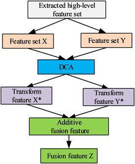
Information fusion can usually be divided into data layer fusion, feature layer fusion and decision layer fusion. Among them, the feature layer fusion is mainly to calculate and process the multi class feature vectors extracted from the original data, so as to realize information fusion. At present, the most classic feature fusion methods based on deep learning models are point-by-point addition (ADD) and vector concatenation (Con-cat) algorithms. ADD could reflect some characteristics of the original features through reducing the parameters and the amount of calculation, but this operation will lead to the loss of some useful information of the original features. The latter concatenates the feature vectors extracted by the network model through the con-cat operation to generate new features directly, and let the network learn without losing information during this process. Although this approach is relatively simple, the two eigenvectors generate redundant information due to their weak correlation, which brings unnecessary increasing in parameters, thus exerting invisible pressure on the network. Therefore, it is not only necessary to analyze the connection and difference between categories while performing feature fusion, but also to consider saving time to improve the performance of the algorithm. To this end, the feature fusion strategy of DCA [26] is introduced. This strategy is improved based on the basis of CCA [27]. While reducing the correlation between features, the redundant correlation between different categories of features is also reduced, so that the feature information extracted in different modes has a better fusion effect to enrich the feature information.

The schematic diagram of the DCA-based feature fusion method is shown in Fig. 1. It is assumed that the extracted two sets of feature matrices are $X$ and $Y$ respectively, and the high level fused feature is $Z$.

First, according to the Eqs. (5) and (6), the average value of the feature vectors within the class ${\overline{x}}_i$ and the average value of the feature vectors between the classes $\overline{x}$ are calculated:

where $x_{ij}\in X$ is the $j$ sample of the $i$ class, $n=\sum _{i=1}^N{n}_i$, $n_i$ is the number of samples of the $i$ class, and $N$ is the number of categories.

Fig. 1Schematic diagram of feature fusion based on DCA

The scatter matrix $S_{bx}$ measuring the relationship between different feature classes can be calculated through ${\overline{x}}_i$ and $\overline{x}$, which is shown in Eq. (7):

where, the matrix ${\mathrm{\Phi }}_{bx}$ is the degree of difference between different categories of features in $X$, and ${{\mathrm{\Phi }}_{bx}}^T{\mathrm{\Phi }}_{bx}$ is the covariance matrix, which is a symmetrical diagonal matrix. Diagonalizing ${{\mathrm{\Phi }}_{bx}}^T{\mathrm{\Phi }}_{bx}$ can make the different categories better separated, that is, $Q^T\left({{\mathrm{\Phi }}_{bx}}^T{\mathrm{\Phi }}_{bx}\right)Q=\mathrm{\Lambda }$, where $Q$ is an orthogonal eigenvector matrix, and $\mathrm{\Lambda }$ is a diagonal matrix of eigenvalues in descending order. The largest non-zero $r$ features can be obtained as following:

Define the transformation matrix $W_{bx}={\mathrm{\Phi }}_{bx}\phi {\mathrm{\Lambda }}^{-1/2}$ to unitize $S_{bx}$, that is, ${W_{bx}}^T{S}_{bx}{W}_{bx}=I$, where $I$ is the inter-class scatter matrix after transformation and dimensionality reduction. The dimensionality of the feature matrix $X$ can be reduced from $p$ to $r$ by $W_{bx}$, as shown in Eq. (10), and this process can reduce the connection between different categories greatly in high-level features:

Similarly, the transformation matrix $Y\text{'}$ of the feature set $Y$ is obtained. In order to enhance the correlation between the corresponding features of the same type in $X$ and $Y$, singular value decomposition (SVD) can be used to diagonalize the inter-class covariance matrix ${S\text{'}}_{xy}=X\text{'}{Y\text{'}}^T$ of $X\text{'}$ and $Y\text{'}$, that is:

where $U$ and $V$ are left and right singular matrices respectively, and $\sum$ is a singular value matrix, which only has a non-zero singular value on the principal diagonal, ${\left(U{\sum }^{-1/2}\right)}^T{S\text{'}}_{xy\left(r\times r\right)}\left(V{\sum }^{-1/2}\right)=I$. The final transform feature sets $X^{\mathrm{*}}$ and $Y^{\mathrm{*}}$ can be obtained through the transformation matrix $W_{cx}=U{\sum }^{-1/2}$, $W_{cy}=V{\sum }^{-1/2}$, as shown in Eqs. (12) and (13):

where $W_x$, $W_y$ are the transformation matrices of high-level feature $X$ and $Y$ respectively. Finally, this paper adopts the addition method for feature fusion as shown in Eq. (14) in order to keep the dimension of the feature vector unchanged:

4. Convolution neural network

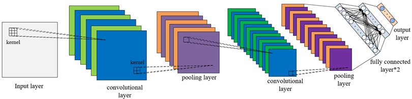
CNN is a multi-level feedforward neural network with strong feature extraction ability, and its network parameters are updated by back propagation algorithm. Typical CNN consists of input layer, convolution layer, pooling layer, FC layer and output layer, in which convolution layer and pooling layer are the core of feature extraction. The convolution layer is connected to the previous layer through local connection and weight sharing, and the convolution operation is carried out to generate features, which reduces the number of required training parameters greatly. The pooling layer extracts deep local features by down-sampling the data dimensions, and reduces the complexity of the network by reducing the required parameters, which not only improves the robustness of the model, but also avoids the overfitting phenomenon effectively. At the same time, it makes easier for CNN to use back propagation algorithms for training. The fully connected layer is mainly used to complete the task of classification or regression, and it has the same structure and calculation method as the traditional feedforward neural network. The basic structure of CNN is shown in Fig. 2.

Fig. 2Typical CNN structure

5. Construction of DCA-CNN network model

5.1. Framework for diagnostic methods

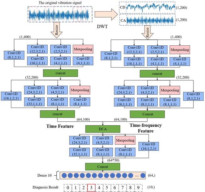
A CNN based intelligent fault diagnosis model by combing with DCA is proposed to solving the problems that limited training data and single input information make feature learning insufficient and low classification accuracy. The model consists of two parallel branches, and each branch is a convolutional pooling extraction process with specific parameters. First, multi-domain feature information of the original signal is extracted by increasing the network’ feature extraction scale. In one branch, the divided training samples in time-domain are processed through the multi-scale CNN branch directly to extract more abundant time-domain feature information. In the other branch, the original training data is transformed by DWT, then further extracts the time-frequency domain feature information of the original data through multi-scale CNN. Subsequently, feature fusion is performed on the extracted multi-domain feature information by DCA feature fusion strategy to enhance the diagnostic performance of the network model. Finally, new features are further extracted from the fused features through a deep multiscale CNN, and the extracted new features are used as the input of the classifier to complete the classification result.

As shown in Fig. 3, the proposed method can be divided into the following four steps:

1) Preprocess the data: the acquired original vibration signal is divided into non-overlapping samples by a sliding window to generate training, validation and test samples.

2) Construct the DCA-CNN network model and set relevant network parameters: number of iteration steps, training batches, number of convolutional layer and so on.

3) Train the Network model: the original training samples are input into the model, and the multi-scale time-domain feature information of the original data training samples is extracted directly through one branch of the multi-scale CNN. At the same time, the training samples handled by DWT are processed by another branch of the multi-scale CNN to extract the multiscale time-frequency feature information. Then, the extracted time-domain and time-frequency domain feature information are fused through the DCA feature fusion strategy to generate fused training features. Finally, the fused training features are further learned and trained through the deep-level of CNN, and the training of network parameters of each layer is completed through iterative training, and finally the trained model is obtained.

4) Input the test sample data into the trained model, and output the classification diagnosis result through the classifier finally.

Fig. 3DCA-CNN network model structure

6. Experiment verification and analysis

In this section, effectiveness of the method is verified through two experiments. In addition, noise interference experiments are carried out and compared with other models to verify the superiority of the proposed model.

6.1. Experiment 1: rolling bearing failure data of case western reserve university (CWRU)

6.1.1. Data description

The experimental data use the rolling bearing fault data set of CWRU [28], and its experimental platform is shown in Fig. 4. The type of bearing selected in the experiment is SKF6205, which is installed on the driving end of the induction motor. The signal is recorded by the accelerometer installed at the drive end of the induction motor, and the data is collected by the 16-channel acquisition instrument, and the sampling frequency is set to 12 kHz. In this experiment, the vibration data set of the first 10 seconds collected by the sensor is selected. In this data set, three types of bearing defects are machined by EDM technology: inner ring, outer ring and rolling body defects. Each type of defect has three different sizes: 0.1778 mm 0.3556 mm and 0.5334 mm. The bearing data of different fault locations and different defect degrees are regarded as one class separately, which includes a total of 10 types. Based on the frequency and rotational speed of the collected data, it can be inferred that the data points collected in each circle are as follows: sampling points (circle) = sampling frequency × 60 / rotational speed = 12000×60 /1797 = 400. Therefore, the sample data is divided by the way of non-overlap. The sample length is set to 400 and the displacement is set to the length of a sample. A total of 3000 samples corresponding to 10 types of bearing states are constructed. The health status is marked with label 0, and the other 9 faults are marked by label 1-9. 70 % of the experimental data set is randomly selected as the training set, 10 % as the verification set, and 20 % as the test set. The details of the sample division of the data set are shown in Table 2.

Fig. 4CWRU bearing fault test rig

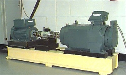
Table 2Sample division of the rolling bearing data set

Fault type	Damage diameter	Sample length	Number of samples	Label
Normal	0	400	300	0
OR007	0.1778	400	300	1
OR014	0.3556	400	300	2
OR021	0.5334	400	300	3
IR007	0.1778	400	300	4
IR007	0.3556	400	300	5
IR007	0.5334	400	300	6
B007	0.1778	400	300	7
B014	0.3556	400	300	8
B021	0.5334	400	300	9

In order to verify the outstanding performance of the proposed network under different load conditions, the original vibration data of the drive bearing under four loads of 0-3hp are selected and defined as data sets A, B, C and D respectively. Each data set contains 10 states, and the description information of the data set is shown in Table 3.

Table 3Dataset description

Data set	Load (hp)	Number of samples /categories	Sample division /categories	Number of categories
A	0	300	7:1:2	10
B	1	300	7:1:2	10
C	2	300	7:1:2	10
D	3	300	7:1:2	10

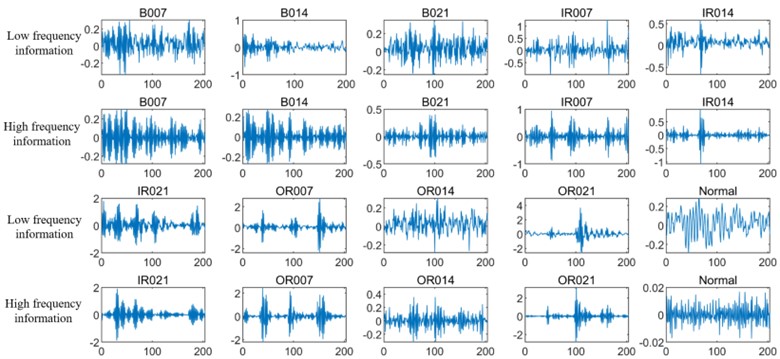
Fig. 5 shows the time domain waveforms of 10 kinds of vibration signals with sample length of 400 under 0 hp load. Based on the proposed DCA-CNN network, the training sample data from the original vibration signal is input to a CNN branch for feature extraction firstly. At the same time, the training data set is transformed by DWT, and then input to another CNN branch for time-frequency domain feature extraction. Fig. 6 shows the low-frequency and high-frequency signals decomposed by DWT. Generally speaking, the low-frequency components usually contain the important characteristics of the signal, while the high-frequency components can show the details or differences of the signal.

Fig. 5Original waveform diagram of bearing vibration signals in different states

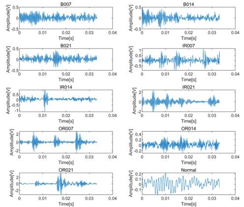
Fig. 6Low-frequency information and high-frequency information of DWT decomposition of bearing vibration signals in different states

6.1.2. Analysis of experimental results

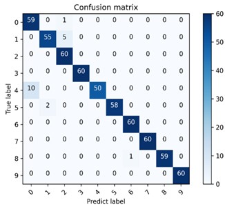
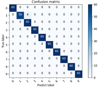
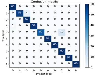
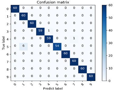
Fig. 7 is one of the confusion matrix diagrams of 10 experiments performed on 4 data sets using the method model in this chapter. The classification accuracy of the diagnostic model on 4 data sets is 97.5 %-99.33 %, among which the classification effect on data set B is the best. The multi-class confusion matrix is able to record the classification results of all conditions in detail, including the classification accuracy and the number of mis-classifications. The dark area on the diagonal of the confusion matrix represents the accuracy rate corresponding to each type of failure, 60 is the number of test sets for each type of failure, and the values in the rest of the area represents the number of misclassifications. The vertical axis is the actual label of the classification, and the horizontal axis is the predicted label of classification. The confusion matrix presented in Fig. 7(b) shows the classification and recognition of the 10 states, and it can be seen from the figure that the model has achieved good classification results under the four types of data sets, indicating that the proposed DCA-CNN diagnosis model has better recognition ability and higher diagnosis accuracy.

Fig. 7The multi-class confusion matrix visualization of the proposed method under 4 data sets

a) Dataset A

b) Dataset B

c) Dataset C

d) Dataset D

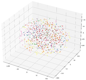
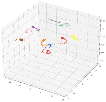
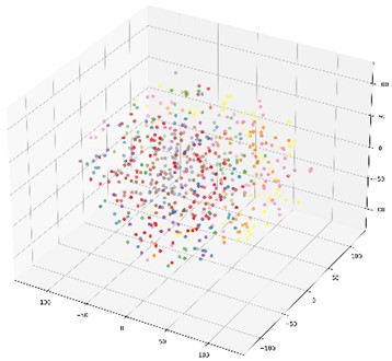
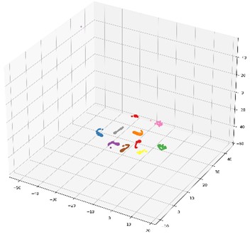
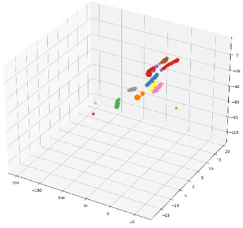
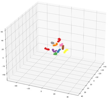
In order to further illustrate the impact of the proposed multi-domain feature fusion strategy on the classification results, the most common t-SNE method in manifold learning is introduced. By mapping high-dimensional feature vectors to three-dimensional space, the t-SNE method is used for dimensionality reduction and feature visualization. Here, it is selected as the feature visualization result graph of the last fully connected layer of the DCA-CNN network model based on data set B, and the corresponding result is shown in Fig. 8(b). Besides, the t-SNE visualization of CNN network model based on data set B is also given in Fig. 8(a) for comparison.

The CNN model compared in this chapter uses the same parameters as the DCA-CNN. It also extracts multiscale time-domain and time-frequency domain features from the original data through two parallel branch CNNs. The difference is that there is no DCA feature fusion in the CNN model. In the process of fusion of CNN, Con-cat is used to fuse the extracted time domain and time-frequency domain features directly. In Fig. 8, the classification accuracy of the test set of the CNN network model is 93.67 %, and the classification accuracy of the DCA-CNN network model is 98.83 %. Compared Fig. 8(b) with Fig. 8(a), the feature classes of the former are more concentrated, and the distance between classes is larger, which proves that the DCA-CNN network model can not only be well clustered into categories, but also easier to be identified.

Fig. 8t-SNE feature visualization

a) CNN network model raw data feature visualization

b) CNN network model last fully connected layer feature visualization

c) DCA-CNN network model raw data feature visualization

d) DCA-CNN network Feature visualization of the last fully connected layer of the model

In the actual operation scene of rotating machinery, environmental noise exists inevitably, and the measured vibration signal is often interfered by noise, which reduces the effectiveness of the fault diagnosis method. In this regard, Gaussian white noise is added into the original data of the test set to simulate the impact of noise on the classification and diagnosis results, and the trained model is used for testing to evaluate the performance of the proposed method in noisy environment. The definition of SNR is shown in Eq. (6):

20

$SN{R}_{dB}=10\mathrm{l}\mathrm{o}{\mathrm{g}}_{10}\left(\frac{P_{\mathrm{s}\mathrm{i}\mathrm{g}\mathrm{n}\mathrm{a}\mathrm{l}}}{P_{noise}}\right),$

where $P_{signal}$ represents the power of the original signal and $P_{noise}$ represents the power of the noise signal. The smaller the SNR, the greater the noise interference.

Fig. 9 shows the test accuracy of the proposed method at different levels of noise compared with the CNN method. It can be observed that adding extra noise usually reduces the diagnostic performance in different scenarios, and stronger noise generally leads to lower test accuracy. Specifically, the model is less accurate when SNR < 2 dB, and is higher than 94 % when SNR > 4 dB. Besides, the proposed method is better than the CNN method in most cases, and high test accuracy can still be obtained in the case of additional environmental noise. It can be seen that the method proposed in this chapter has strong anti-noise stability and generalization ability.

Fig. 9Accuracy rate of rolling bearing test set under different SNR

6.1.3. Comparison

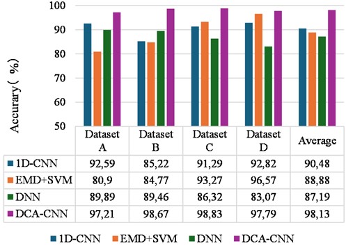
For the method proposed in this study, several conventional bearing fault recognition models are used for comparison: 1D-CNN [29], EMD+SVM [30], DNN network [31]. Here, 1D-CNN directly trains and tests the original signal data set in time domain. EMD+SVM decomposes the input vibration signal by using EMD, and then uses fuzzy entropy to extract the characteristics of the vibration signal effectively. The DNN uses nine time-domain statistical features of the original as input. This test is divided into 4 groups to verify the diagnostic performance of the proposed network under different load conditions. At the same time, the above conventional fault identification methods were tested on various data sets for 10 times in order to reduce the interference of uncertain factors on the experimental results and ensure the reliability of the proposed method, and the average value was taken as the final diagnostic accuracy. Fig. 10 shows the average recognition accuracy trend graph of the different methods under different data sets.

Fig. 10The average recognition accuracy of different methods under different data sets

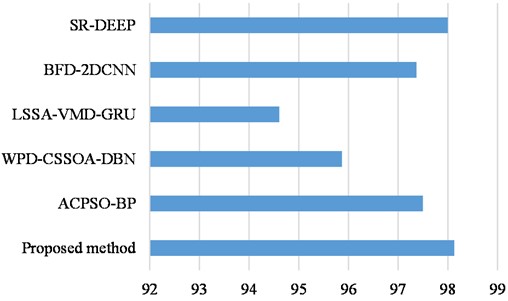
To verify the superiority of the method, we compared it with the advanced methods: (1) SR-DEEP [32], (2) BFD-2DCNN [33], (3) LSSA-VMD-GRU [34], (4) WPD-CSSOA-DBN [35], (5) ACPSO-BP [36]. The experimental results are shown in Fig. 11.

From the results as shown in Fig.10, it can be seen that the 1D-CNN model and the DNN diagnostic model have relatively stable diagnostic performance under the 4 datasets, but their diagnostic accuracies are low. EMD+SVM has a better diagnostic performance on the data set D, but has the worst diagnostic accuracy on dataset A. From the results as shown in Fig. 11, our proposed method achieves optimal results. Furthermore, the DCA-CNN diagnostic model proposed in this chapter has achieved relatively good diagnostic accuracy in the four types of data sets, and its average recognition accuracy and recognition accuracy of each data set are basically higher than other methods.

Fig. 11The average recognition accuracy of different methods

6.2. Experiment 2: gearbox failure data of QPZZ-II test bench

6.2.1. Description of experimental data

The gear fault vibration signals collected from the QPZZ-II rotating machinery vibration test bench [37] is used to further verify the proposed method, and Fig. 12 shows the experiment rig. Ten different kinds of gear failures are simulated on the test bench, and the teeth numbers of the test gears are 75 and 55 respectively. The modulus of the test gears is 2. In the experiment, the wire EDM process was used to create faults in the large gear. By replacing the faulty gear in the gear box, a total of 10 different gear states were simulated, and their corresponding faulty parts are shown in Fig. 13. Vibration data in different states are collected through an acceleration sensor installed on the gearbox. The motor speed is 1500 r/min, the sampling frequency is set to 12,800 Hz, and the sampling time is set as 10 s. A total of 128,000 data points are obtained for each state. In the experiment, 400 data points were selected as the data of one sample, and the number of samples for each type of fault was 320 using non-overlapping division. The sample was divided into training set, verification set and test set according to the ratio of 7:1:2. Table 4 shows the details of the ten running states. The original waveforms of the ten kinds running states and their corresponding decomposed low-frequency signal components and high-frequency signal components using DWT are presented in Fig. 14 and Fig. 15 respectively.

Fig. 12QPZZ-Ⅱ rotating machinery vibration test bench

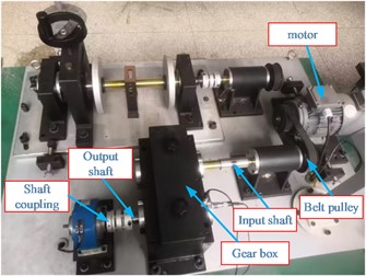
Fig. 13Gear failure parts

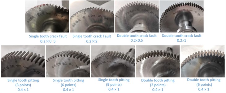
Fig. 14Original waveform diagram of gear vibration signal in different states

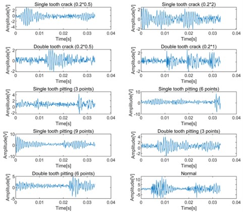
Fig. 15Low-frequency information and high-frequency information of DWT decomposition of gear vibration signals in different states

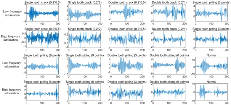
Table 4Gear failure dataset description

Fault type	Failure points	Damage diameter	Sample length	Number of samples	Sample division	Label
Normal	–	–	400	320	224/32/64	0
Single tooth crack fault	–	0.2×0.5	400	320	224/32/64	1
	–	0.2×2	400	320	224/32/64	2
Double tooth crack fault	–	0.2×0.5	400	320	224/32/64	3
	–	0.2×1	400	320	224/32/64	4
Single tooth pitting fault	3 Point	Ø0.4×1	400	320	224/32/64	5
	6 Point	Ø0.4×1	400	320	224/32/64	6
	9 Point	Ø0.4×1	400	320	224/32/64	7
Double tooth pitting fault	3 Point	Ø0.4×1	400	320	224/32/64	8
	6 Point	Ø0.4×1	400	320	224/32/64	9

6.2.2. Analysis of experimental results

The accuracy curves using the proposed method and CNN network directly are shown in Fig. 16 after conducting 10 experiments, and their average accuracy ratios are 98.96 % and 95.41 % respectively. The advantage of the proposed method over the CNN network is verified. The multi-class confusion matrix and t-SNE feature visualization of the results obtained in the fourth of 10 experiments using the proposed method and CNN model are given in Fig. 17 and Fig. 18 respectively, and their recognition accuracy rates are 99.69 % and 94.84 % respectively, which further verify the effectiveness of the proposed method intuitively.

Fig. 16Test set accuracy for ten trials

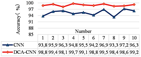
Fig. 17The proposed method is used to visualize the multi-class confusion matrix under the gear dataset

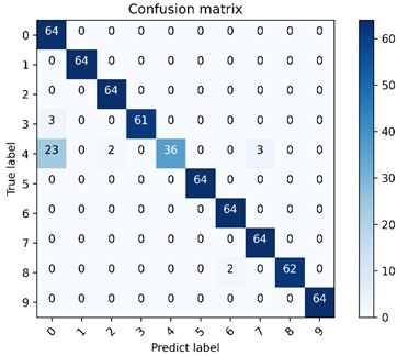
a) CNN network model multi-class confusion matrix visualization

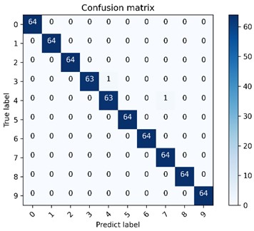
b) DCA-CNN network model multi-class confusion matrix visualization

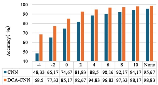
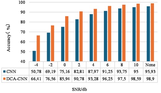
By adding noise interference with different degree of SNRs to the gear test set data, the diagnostic effect of the method on the gear fault data set under the noise interference is verified. Accordingly, the noise interference on the CNN model method is compared, and the results are shown in Fig. 19. It can be seen from the figure that when the SNR is –4 dB, the classification accuracy of the CNN model is 50.78 %, while the classification accuracy of the DCA-CNN model is 66.41 %. When the SNR becomes 6dB, the classification accuracy of the DCA-CNN model can reach more than 96 %, which shows the effectiveness of the model for fault diagnosis of gearboxes in noisy environments.

Fig. 18The proposed method is used for t-SNE feature visualization under the gear dataset

a) Feature visualization of the last fully connected layer of the CNN network model

b) Feature visualization of the last fully connected layer of the DCA-CNN network model

Fig. 19Accuracy of gear test set under different SNR

6.2.3. Comparison

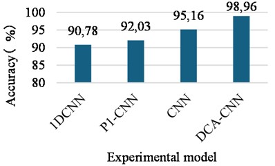
Similarly, 1DCNN, P1-CNN, CNN, and DCA-CNN were used to conduct ten experiments on the gearbox fault data set for comparison, and their corresponding average values are used as the final accuracy. Among them, the 1DCNN model adopts the five-layer convolution and pooling layer structure built in Chapter 3 in this paper. The P1-CNN model is constructed by combining the time-domain multi-scale feature extraction with deep multi-scale feature extraction part of the DCA-CNN model. The CNN model is constructed by combining the multi-domain and multi-scale feature extraction part of the DCA-CNN model with the deep multi-scale feature extraction part, in which the multi-domain feature is not fused by DCA, but a simple concept operation is used.

As can be seen from Fig. 20, P1-CNN model does not need a deeper network structure to achieve higher diagnostic accuracy than 1DCNN model due to the addition of multi-scale feature extraction module. CNN model has higher diagnosis accuracy than 1DCNN and P1-CNN model due to the adding multi-domain feature extraction module and multi-scale feature extraction module. The diagnostic accuracy of DCA-CNN model is the highest, which is 98.96 %. These show that the method proposed in this chapter can improve the diagnosis performance of CNN network effectively through multi-scale feature extraction module, multi-domain feature extraction module and feature fusion module based on DCA. Besides, the proposed method also could achieve higher classification diagnosis accuracy when the input data is relatively single and the actual data set is limited.

Fig. 20The average accuracy of the gear failure test set under different methods

7. Conclusions

In this paper, a network model based on DCA and CNN is proposed for fault diagnosis of rotating machinery. The following conclusions could be obtained according to the analysis of two groups of different types of experimental data by using the proposed method:

1) Through the combination original signal processing handling ability of DWT with the strong nonlinear feature learning ability of CNN, the proposed method can get rid of the dependence on signal processing technology and manual feature extraction and can extract effective deep fault features adaptively and improve the diagnosis accuracy of the model.

2) The most representative feature information could be obtained by adding the DCA feature fusion module into the multi-domain CNN network model to fuse the extracted multi-domain feature information. Meanwhile, the correlation between similar fused features is improved, and the redundant correlation between different types of features is reduced.

3) Compared with series of other fault diagnosis methods, the results show that the proposed model can still achieve higher diagnosis in the case of limited data set and single input information and has a wide range of application. Besides, the anti-noise performance of the proposed model is verified.

In the future work, we will verify the scalability of the proposed DCA-CNN diagnosis model on a large-scale equipment. In addition, we will further study the fault diagnosis of rotating machinery under variable working conditions based on this method and study the applicability of fault diagnosis based on two-dimensional image data, so as to further improve the performance of the proposed model.

As for the engineering application of the proposed method, it could be embedded as an algorithm package into the device online monitoring software, and the algorithm package only needs to define the input and output. The proposed method can also be embedded as algorithm package into offline monitoring instruments to service the low-cost offline monitoring instrument users. Of course, as the proposed method is developed based on Matlab and Python languages, both software engineering and hardware engineering applications cannot be separated from the mixing programming of Matlab, Python with other development languages such as C++ and Java.