Abstract
A fault diagnosis method for the rotating machinery based on improved Convolutional Neural Network (CNN) with Gray-Level Transformation (GLT) is proposed to increase the accuracy of the recognition adopting the multiple sensors. The Symmetrized Dot Pattern (SDP) in this method is applied to fuse the data of the multiple sensors, and the multi-color value method is adopted to increase the feature dimension. The grayscale and GLT are used to reduce the dimension of the SDP image. The SDP grayscale image is finally input to the CNN network for training recognition. The research results show that the diagnosis accuracy of the rolling bearing system based on the novel method is up to 98.6 %. Compared with the method without the multi-color value and GLT, the recognition accuracy of the proposed method is improved by 22.3 %, and the training time is reduced by about one third. The research work reveals that the developed method has the potential application value under the multi-sensor working conditions for the fault diagnosis.
Highlights
- A fault diagnosis method for the rotating machinery based on improved Convolutional Neural Network (CNN) with Gray-Level Transformation (GLT) is proposed
- The Symmetrized Dot Pattern (SDP) is applied to fuse the data of the multiple sensors, the multi-color value method is adopted to increase the feature dimension and the grayscale and GLT are used to reduce the dimension of the SDP image
- The diagnosis accuracy of the rolling bearing system based on the novel method is increased
1. Introduction
Rotating machinery has a wide range of applications in aviation, the railways, the shipping, the electric power and the other fields. In these fields, a lot of manpower and material resources are spent to fix the position of the mechanical faults. Therefore, it is essential to develop a convenient and accurate method of the fault diagnosis for the rotating machinery.
In recent years, technologies related with the deep learning have developed rapidly, and the researchers have obtained world-renowned achievements in the image recognition, the natural language recognition and the other fields [1]-[5]. Guo et al. [6] proposed a diagnosis method that uses a Convolutional Neural Network to directly classify the continuous wavelet transform scale map of the rolling bearing vibration signals. Xie et al. [7] developed an adaptive deep belief network model to achieve end-to-end fault diagnosis, the model is adopted to extract the deep representative features from the rotating machinery and to identify the bearing fault types and the fault levels. Landauskas et al. [8] proposed a bearing fault diagnosis method based on the classification of the patterns for the permutation entropy and these patterns are interpreted, processed and classified by employing deep learning techniques based on the Convolutional Neural Networks. Lee et al. [9] proposed a transfer learning network based on the multi-objective instance weighting, they solved the problem of the negative transmission and successfully applied the method to fault diagnosis. Li et al. [10] proposed a fault diagnosis method based on short-time Fourier transform and Convolutional Neural Network for realizing the end-to-end fault pattern recognition. A method combining the Wavelet Transform (WT) and the Deformable Convolutional Neural Network (D-CNN) is proposed to realize accurate real-time fault diagnosis of the end-to-end rolling bearing [11]. Shao et al. [12] presented a convolutional deep belief network for the bearing fault diagnosis of the electric locomotives. Xu et al. [13] combined the SDP method and the matching image to detect the centrifugal fan stall in the real time. Chen et al. [14] developed a rolling bearing fault diagnosis method applying the graph spectrum amplitude entropy of the visibility graph (GSAEVG) and presented a rolling bearing fault diagnosis based on the graph spectrum amplitude entropy of the visibility graph (GSAEVG) method. Zhu et al. [15] converted the one-dimensional (1-D) vibration signal measured by the sensor into a two-dimensional (2-D) gray image as the network input. Zhao et al. [16] proposed signal-to-image mapping (STIM) to convert the one-dimensional vibration signals into two-dimensional grey images. Fu et al. [17] used different sizes of one-dimensional convolution kernels to extract the multi-scale features and the multi-layer network learning from the original vibration signal, realizing the intelligent fault diagnosis. Chen et al. [18] applied the diagonal slice spectrum (DSS) to the final signal of ATVMF, the method enhanced the pulse characteristics related to the fault and can diagnose the weak fault of the bearing. A new fault diagnosis method based on the Wavelet Transform (WT), the Principal Component Analysis (PCA) and the autocorrelation noise reduction effectively is developed to extract the characteristic frequency of the rolling bearing combined faults [19]. A novel fault diagnosis approach based on the improved Manhattan distance in Symmetrized Dot Pattern (SDP) image is proposed. In this way, the improved Manhattan distance between the local matrix of each IMF components and corresponding mean matrix is extracted. Different vibration signal of rolling bearing is classified according to this improved Manhattan distance [20]. Sun et al. [21] used the Symmetrical Dot Plot (SDP) method to preserve and convert the eigenmode function (IMF) components. After positioning each SDP image through binarization, the local SDP images are averaged to obtain the mean image as a benchmark. TSFFCNN-PSO-SVM can identify fault modes from the vibration signals more accurately with fewer iterations at the same time. The Two-Stream Feature Fusion Convolutional Neural Network (TSFFCNN) is established. In-depth features are extracted from the proposed parallel multi-channel structure of 1D-CNN and 2D-CNN [22]. Li et al. [23] calculated the morphological spectrum entropy by obtaining the morphological spectrum of the fault signal and described the morphological characteristics of the different signals of the rolling bearing. Wang et al. [24] proposed the method based on the Symmetrized Dot Pattern (SDP) analysis and improved Back Propagation (BP) neural network to accurately diagnose the mechanical failure of fan. Zan et al. [25] developed a fault diagnosis model of the rolling bearing based on the multi-input layer convolutional neural network, the research work improved the recognition accuracy of the model and anti-interference ability. Zhu et al. [26] transformed the multiple vibration signals into the Symmetrized Dot Pattern (SDP) images, and then identified the SDP graphical feature, which improved the rotor fault diagnosis accuracy. Li et al. [27] combined the adaptive symmetric point mode and the density-based spatial clustering with the noisy applications to reduce the impact of noises on the diagnostic accuracy.
In terms of the multi-sensor data fusion, a multi-sensor data fusion classification method based on the Linear Discriminant Analysis (LDA) is presented [28]. The Dempster-Shafer (D-S) evidence theory is used to fuse the multi-sensor data to improve the diagnostic accuracy [29].
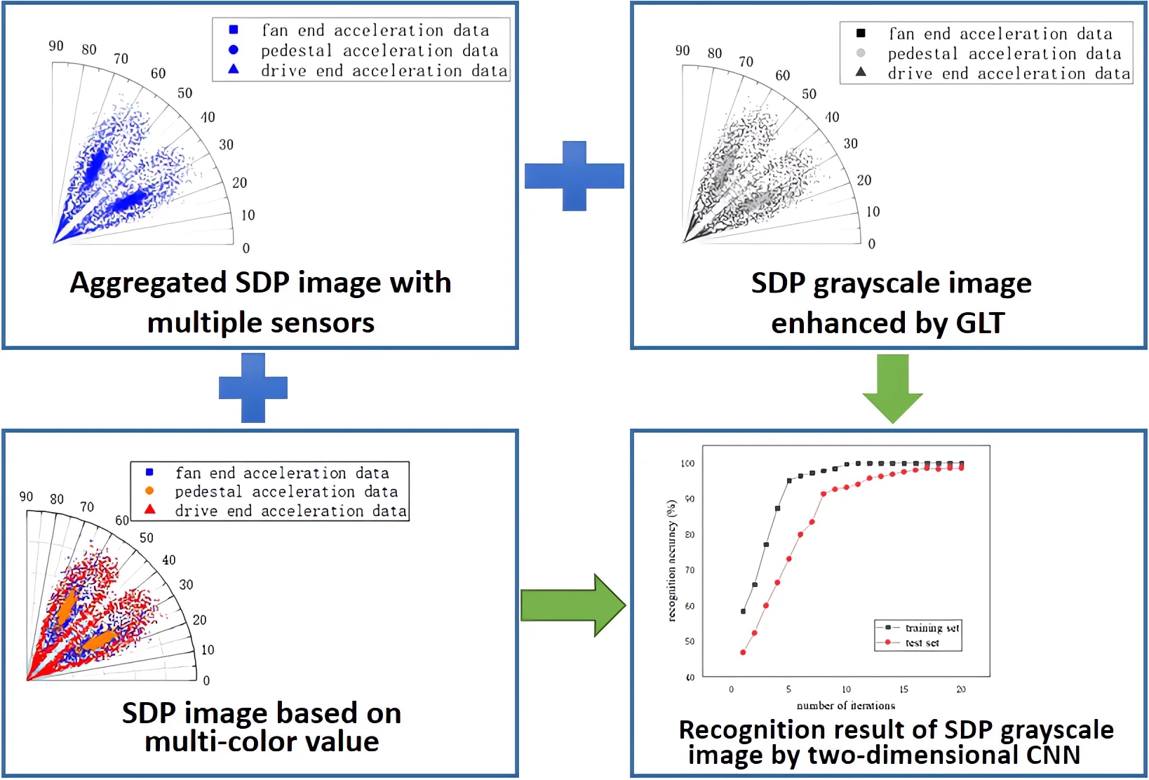
Most of researches using a single or a small number of sensors are carried out. However, the number of sensors in the actual working conditions is enormous. Using the above research methods to diagnose the faults of rotating machinery will result in insufficient use of the sensor data. In addition, the sensor type selected for the fault diagnosis cannot reflect the characteristics of the fault well, which will affect the accuracy of fault diagnosis. Therefore, the CNN, SDP and GLT are introduced to develop a novel fault diagnosis method for accuracy. In this method, the feature data of multiple sensors are aggregated into one spatial dimension, and the SDP images is generated, the multi-color value method is adopted to increase the dimension of the feature data and to reduce the amount of calculation through the grayscale and GLT, and finally the SDP images is transferred to the CNN network for training recognition.
2. SDP analytical method
In the existing signal analysis methods of the bearing vibration, the time domain, the frequency domain or the time-frequency domain data are studied by a single sensor. In the SDP method, the time-domain data of the multiple sensors can be mapped as a two-dimensional SDP image through certain calculations, the image can show the characteristics of the time-domain data through the spatial information, and finally the image can be analyzed and recognized to achieve the purpose of diagnosing bearing faults.
2.1. SDP formulation
The time domain signal in the data set, , can be converted into the corresponding point in polar coordinates through the SDP formula.
The SDP formula is as follows:
where is the maximum value in the time domain signal of the data set; is the minimum value in the time domain signal of the data set; is the number of the time intervals between two nodes corresponds to the number of points in the data set; is the rotation angle of the mirror symmetry plane (the value is 360 m/n, 1, 2,..., ); is the magnification factor, when the value is too large, the data in different data sources will affect each other, and too small value will result in the inconspicuous features, so it needs to be selected after the experiments. In Fig. 1, represents the radius of the transformed coordinates of the data in the polar coordinate system; means the deflection angle of the coordinate in the counterclockwise direction; is the deflection angle of the coordinate in the clockwise direction, as shown in Fig. 1.
Fig. 1Schematic diagram of SDP

2.2. Selection of parameters
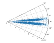
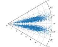
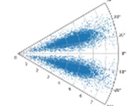
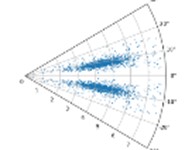
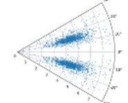
On condition of using the drive end fault, the SDP images generated by the bearing vibration signal is elected in this section when the value of is 10, 30, 60, and is equal to 10°, 20°, and 30°.
In the case of constant , with the increase of , the higher the degree of aggregation of the characteristic data of the sensor in the SDP image, this is not conducive to distinguishing the characteristics of the different types of faults. When is constant, with the increase of , the shape of the graphic arm in the SDP image and the distance between the two graphic arms are larger, and the characteristics of the fault data can be better displayed, as shown in Fig. 2. Therefore, = 10 and = 30° are used in the subsequent CNN training.
Fig. 2SDP images when l is 10, 30,60, and ξ is 10°, 20°, and 30° respectively under drive-end fault
a) 10; 10°
b) 10; 20°
c) 10; 30°
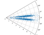
d) 30; 10°
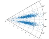
e) 30; 20°
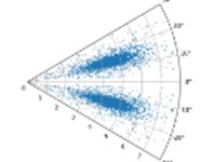
f) 30; 30°
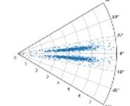
g) 60; 10°
h) 60; 20°
i) 60; 30°
3. Grayscale method and GLT
3.1. Grayscale method
There are three commonly used grayscale methods, the maximum value method, the average value method, and the weighted average method. The maximum method is to obtain the value of R, G and B values of the pixel, and then take the maximum value, similar to the maximum pooling:
The average of R, G and B is taken in the average method:
A certain weight is introduced to weight the values of R, G and B in weighted average method:
where , , refer to the weighted value of R, G, B, respectively. For the weighted average method, because the human eye is more sensitive to the green color and least sensitive to the blue color, accordingly = 0.299, = 0.578 and = 0.114 are selected in the related research. After a large number of tests, the weighted average method is the best in the SDP image recognition, therefore, the weighted average method is adopted in this research work.
3.2. GLT
Gray Level Transformation method is applied to enhance SDP gray image in this study. GLT strengthens or suppresses the grayscale of each pixel through the different strategies. There are three commonly used gray-scale transformation methods, namely the linear gray-scale transformation, the exponential gray-scale transformation and the logarithmic gray-scale transformation [30]. The piecewise linear transformation in the linear gray scale transformation is applied in this study.
The R, G and B values of each pixel in the grayscalized image are the same, ranging from 0 to 255. In order to highlight or suppress a certain color, the gray level corresponding to the color can be mapped to a higher or lower interval by the linear transformation:
where and are the mapping parameter values in the different intervals respectively.
4. CNN network model
Convolutional Neural Network is a feedforward neural network consisting of one or more convolutional layers, the pooling layers and the fully connected layers. Through this structure, the data characteristics can be extracted by using the two-dimensional structure of the input data. Therefore, it is widely used in the field of image recognition [31]. The model consists of three convolutional layers, three pooling layers and three fully connected layers. The number of convolution kernels in the convolution layer respectively is 32, 64 and 64. All the convolution kernel’s size of these convolution layers are 5×5, 5×5, 5×5. The pooling layers are all the largest pooling layers, and their size is 2×2. In this paper, the convolution layer and the first two full connection layers use the relu activation function, and the last layer uses the softmax function and the cross entropy loss function. The relu activation function and softmax activation function are shown in Eqs. (8) and (9), respectively:
where is the result after the calculation through the activation function; is the output of the previous layer.
The cross entropy loss function is shown in Eq. (10):
where is the number of the categories to be classified; is the indicator variable, it is equal to 1 when the specimen is consistent with the category, and it is 0 when the specimen is inconsistent with the category; is the predicted probability of the category for the input specimen.
See Table 1 for network structure parameters.
Table 1Network structure parameters
Network layer name | Parameter | Output feature size |
Input layer | – | (12000, 480, 640, 1) |
Convolutional layer C1 | (32, 5, 5) | (None, 480, 640, 32) |
Activation function | Relu | – |
Pooling layer P1 | (2, 2) | (None, 240, 320, 32) |
Convolutional layer C2 | (64, 5, 5) | (None, 240, 320, 64) |
Activation function | Relu | – |
Pooling layer P2 | (2, 2) | (None, 120, 160, 64) |
Convolutional layer C3 | (64, 5, 5) | (None, 120, 160, 64) |
Activation function | Relu | – |
Pooling layer P3 | (2, 2) | (None, 60, 80, 64) |
Flatten layer | – | (None, 207200) |
Fully connected layer F1 | – | (None, 512) |
Activation function | Relu | – |
Fully connected layer F2 | – | (None, 128) |
Activation function | Relu | – |
Fully connected layer F3 | – | (None, 10) |
Activation function | Softmax | – |
5. Rotating machinery fault diagnosis
5.1. Data source
The bearing vibration data set of CWRU is recognized by academia. A lot of highly cited papers use this data set for the calculation and analysis. Therefore, in order to facilitate comparison with the results of other research, this data set is used in this article for training.
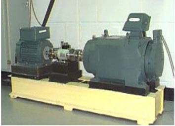
The device is mainly composed of the fan end, the drive end and the pedestal, as shown in Fig. 3. There are respectively the acceleration sensor on the fan end, the drive end and the base. The vibration acceleration signal of the bearing is obtained by a 16-channel data recorder under no load, 1 HP, 2 HP, and 3 HP (horsepower). The sampling frequency of different positions is diverse. The sampling frequency of the fan end is 12 KHz, and the sampling frequency of the drive end is 12 KHz and 48 KHz. The bearing is a deep groove ball bearing of model SKF6205, and the fault on the bearing is a single point damage caused by the electric spark. In addition to the fault location, the bearing fault characteristics also include the fault width. The EDM machined the faults with widths of 0.007 inches, 0.014 inches and 0.021 inches respectively
Fig. 3CWRU data set collection device
In order to facilitate the calculation, the bearing vibration signals are all normalized:
where is the minimum value of signal; is the maximum value of signal; is the signal value to be normalized; is the value after the normalization.
In this paper, the sampling rate of the 12 K drive end is 12000 / s. For the different fault depths and the different loads, there are 120984 data in each MATLAB data set, which is the data collected within 10 s. The bearing speed is about 1800 rpm, therefore there are about 300 cycles of data in 10 s. The data of each cycle is a specimen; and there are 12000 specimens in total. These specimens are respectively come from no fault, the inner ring fault with 0.007 inch, the inner ring fault with 0.014 inch, the inner ring fault with 0.021 inch, the ball fault with 0.007 inch, the ball fault with 0.014 inch, the ball fault with 0.021 inch, the outer ring fault with 0.007 inch, the outer ring fault with 0.014 inch and the outer ring fault with 0.021 inch. Each fault type is divided into 200 training sets and 100 validation sets, as shown in Table 2.
Table 2Bearing vibration data used by CNN-based SDP image recognition network
Bearing status | Fault size (inch) | Number of specimens | Category number | |||
0 HP | 1 HP | 2 HP | 3 HP | |||
No fault | 0 | 300 | 300 | 300 | 300 | 1 |
Inner ring failure | 0.007 | 300 | 300 | 300 | 300 | 2 |
0.014 | 300 | 300 | 300 | 300 | 3 | |
0.021 | 300 | 300 | 300 | 300 | 4 | |
Ball fault | 0.007 | 300 | 300 | 300 | 300 | 5 |
0.014 | 300 | 300 | 300 | 300 | 6 | |
0.021 | 300 | 300 | 300 | 300 | 7 | |
Outer ring fault | 0.007 | 300 | 300 | 300 | 300 | 8 |
0.014 | 300 | 300 | 300 | 300 | 9 | |
0.021 | 300 | 300 | 300 | 300 | 10 | |
Number of samples | 3000 | 3000 | 3000 | 3000 | ||
5.2. SDP image generation
Zhu et al. [32] let 60°, 150°, 240°, 330° to generate SDP images, which is equivalent to acquiring and mapping four different types of sensor data onto SDP images. However, in the actual production environment, there may be more than four sensors to collect relevant data. When = 30 is a constant, there may not be enough space in the SDP image to display the data of each sensor.
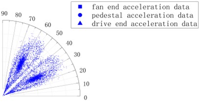
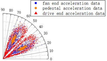
In order to simulate the actual production situation as much as possible, the most extreme method of the parameter selection is adopted. The acceleration data for the fan end, the driving end and the pedestal are uniformly used to draw the SDP image with 45°. For the actual working conditions, regardless of the number of sensors, it can be expressed by using the SDP image generated by this parameter. At this time, the data of the three sensors are completely aggregated and the features between them are in a state of confusion. It is necessary to segment the data of different types of sensors from other dimensions of the image, as shown in Fig. 4.
Fig. 4Aggregated SDP image under the same θ with multiple sensors
For an image, in addition to the features in the spatial dimension, the color value is also vital. Therefore, for the data output by different sensors, the dimension of the feature can be increased by assigning the different color values to it. In order to make the difference between the data characteristic output by the different sensors more sensitive, it is necessary to select color values with the larger differences in R, G and B values. After the comparison of the various color combinations, the orange (255, 165, 0), the blue (0, 0, 255) and the red (255, 0, 0) are selected for the multi-color valuation, the color combination can more meet the requirement of the difference between the data characteristics.
Although the data output by the three types of sensors are at the same location in space, by assigning the different color values to them, the data on the fan end, the pedestal and the drive end. Can be clearly distinguished, as show in Fig. 5.
Fig. 5SDP image based on multi-color value
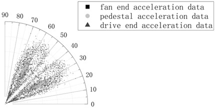
Because three colors of blue, orange and red is used to represent three different types of the data sources, and the RGB values calculated by the weighted average method respectively are 176.615, 29.07, and 76.245. Taking 50, 150, 0.5, 1, = 1.2 and the piecewise linear transformation is applied to the SDP image with the multi-color values.
In this grayscale image, the data of the three types of sensors can be clearly distinguished, it indicates that the grayscale and GLT can enhance the feature difference between the different types of data while reducing dimensionality, as shown in Fig. 6.
Fig. 6SDP grayscale image enhanced by GLT
5.3. Diagnosis results
The CNN network is used to train and recognize the SDP grayscale images, as shown in Table 1. After 20 iterations, the recognition accuracy of the network on the training set reaches up to 100 %, and the recognition accuracy on the test set reaches up to 98.6%, as shown in Fig. 7.
The diagnostic accuracy of this model for the inner ring faults and no faults is 100 %. When the ball is faulty and the fault depth is 0.007 inches, there is a 97 % recognition accuracy. When the fault depth is 0.014 inches, there is a 99 % recognition accuracy. When the fault depth is 0.021 inches, there is a 98 % recognition accuracy. When the outer ring is faulty and the fault depth is 0.007 inches, there is a 97 % recognition accuracy. When the fault depth is 0.014 inches, there is a 98 % recognition accuracy, and when the fault depth is 0.021 inches, there is a 97 % recognition accuracy. To sum up, it shows that this method has high recognition accuracy and has a certain feasibility in the diagnosis of rotating machinery faults. As shown in Table 3.
Fig. 7Recognition result of SDP grayscale image by two-dimensional CNN network CNN network
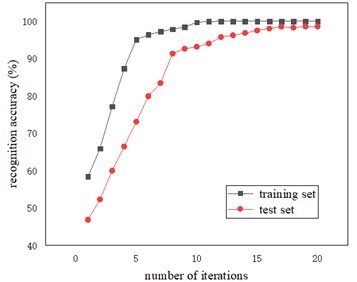
Table 3Diagnosis accuracy under different types of faults
Category number | Test specimen / test set | Error specimen / test set | Recognition accuracy |
1 | 100 | 0 | 100 % |
2 | 100 | 0 | 100 % |
3 | 100 | 0 | 100 % |
4 | 100 | 0 | 100 % |
5 | 100 | 3 | 97 % |
6 | 100 | 1 | 99 % |
7 | 100 | 2 | 98 % |
8 | 100 | 3 | 97 % |
9 | 100 | 2 | 98 % |
10 | 100 | 3 | 97 % |
5.4. Visualization of convolutional layer output
The bearing vibration signal characteristics of the different types of the faults in the input data are aggregated together, and it is difficult to distinguish what fault a bearing vibration signal is. In order to identify the fault features, the vibration signal is converted to 2-Dimensional visual signal, seen in Fig. 8(a); the signal was then extracted through multiple convolutional layers. After the first layer of convolutional layer feature extraction, the 0.007 inches inner ring fault and the 0.007 inches outer ring feature are extracted, but the features of other types of faults are still aggregated together, as seen in Fig. 8(b). After the second convolutional layer is extracted, it can be clearly seen that the characteristics of each type of fault have been separated, but the 0.014 inches outer ring fault and the 0.014 inches rolling element fault are relatively close, there is still the possibility of misjudgment, as shown in Fig. 8(c). After the third convolutional layer is extracted, the characteristics of each type of fault are completely separated and have favorable cohesion, as shown in Fig. 8(d). The last layer of fully connected layer maps each feature data to a one-dimensional space, so the two-dimensional display also tends to a straight line, as shown in Fig. 8(e).
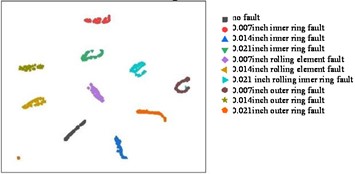
5.5. Comparison with other diagnostic methods
In order to compare with the other diagnostic methods and verify the advantages of the method proposed in this article in recognition accuracy and training time, the results of the method using GLT and the method without using GLT will be compared when the input data is an SDP image without the excessive color value and the grayscale processing. At the same time, the results of this method are compared with the results of SVM, DBN and RNN neural networks when the input data is an SDP image that has been multi-color valued, grayed out and enhanced by the GLT.
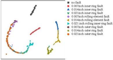
The two-dimensional visualization of the last full connection layer without using the GLT method shows that various faults are difficult to distinguish. There are three examples, 0.007 inches rolling body failure and 0.007 inches outer coil failure, 0.014 inches inner ring failure and 0.014 inches rolling body failure, 0.021 inches inner coil failure and 0.021 inches rolling body failure and 0.021 inches outer coil failure, indicating that no GLT method is not suitable for many sensors, as shown in Fig. 9.
Fig. 8Visualization of convolutional layer output
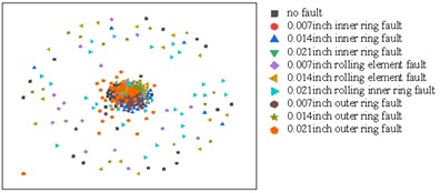
a) Two-dimensional visualization of input data
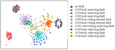
b) Visualization of the output of the first convolutional layer
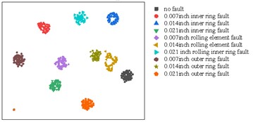
c) Visualization of the output of the second convolutional layer
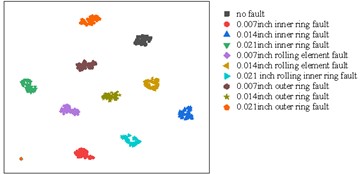
d) Visualization of the output of the third convolutional layer
e) Visualization of the output of the last fully connected layer
Fig. 9Visualization of the output of the last fully connected layer without using the GLT method
In order to illustrate the superiority of CNN-GLT-SDP method, we compare the accuracy and single iteration time of 1070 training machine diagnosis under the same training set and verification set with CNN diagnosis method without GLT and SVM, DBN and RNN methods with GLT.
The results show that the diagnosis method based on CNN-GLT-SDP has not only higher accuracy than other methods, but also takes less time for a single iteration than the other methods. The detailed results are shown in Table 4.
Table 4Comparison of recognition accuracy and single iteration duration of different models
Model type | Test set recognition accuracy | Time required for a single iteration (min) |
Fault diagnosis method without GLT | 77.3 % | 204.1 |
Fault diagnosis method using GLT | 98.6 % | 147.3 |
SVM | 83.62 % | 162.8 |
DBN | 94.58 % | 215.9 |
RNN | 93.26 % | 183.2 |
6. Conclusions
Aiming at the problem of fault diagnosis of the rotating machinery, a fault diagnosis method based on CNN-SDP-GLT is proposed in this paper. The SDP method is used to mix data from the different sensors. The multi-color value method is used to increase the feature dimension. The GLT method is used to reduce the dimensionality and reduce the amount of calculation. Experimental results show that compared with other methods, the method proposed in this paper can use the data from the multiple sensors; and the approach has the higher recognition accuracy and the shorter single iteration time. This method has a reference significance for the fault diagnosis of the rotating machinery under actual working conditions. The data used in this method is not the data under the actual working conditions, therefore the effects of noise and the other effects are not taken into account. In the future, the further research will be conducted on the fault diagnosis under the noise pollution.
References
-
S. Levine, P. Pastor, A. Krizhevsky, J. Ibarz, and D. Quillen, “Learning hand-eye coordination for robotic grasping with deep learning and large-scale data collection,” The International Journal of Robotics Research, Vol. 37, No. 4-5, pp. 421–436, Apr. 2018, https://doi.org/10.1177/0278364917710318
-
D. S. Kermany et al., “Identifying medical diagnoses and treatable diseases by image-based deep learning,” Cell, Vol. 172, No. 5, pp. 1122–1131.e9, Feb. 2018, https://doi.org/10.1016/j.cell.2018.02.010
-
T. Young, D. Hazarika, S. Poria, and E. Cambria, “Recent trends in deep learning based natural language processing,” arXiv:1708.02709, 2017.
-
T. Young, D. Hazarika, S. Poria, and E. Cambria, “Recent trends in deep learning based natural language processing,” IEEE Computational Intelligence Magazine, Vol. 13, No. 3, pp. 55–75, Aug. 2018, https://doi.org/10.1109/mci.2018.2840738
-
S. Bianchi, A. Corsini, A. G. Sheard, and C. Tortora, “A critical review of stall control techniques in industrial fans,” ISRN Mechanical Engineering, Vol. 2013, pp. 1–18, Jun. 2013, https://doi.org/10.1155/2013/526192
-
S. Guo, T. Yang, W. Gao, and C. Zhang, “A novel fault diagnosis method for rotating machinery based on a convolutional neural network,” Sensors, Vol. 18, No. 5, p. 1429, May 2018, https://doi.org/10.3390/s18051429
-
J. Xie, G. Du, C. Shen, N. Chen, L. Chen, and Z. Zhu, “An end-to-end model based on improved adaptive deep belief network and its application to bearing fault diagnosis,” IEEE Access, Vol. 6, pp. 63584–63596, 2018, https://doi.org/10.1109/access.2018.2877447
-
M. Landauskas, M. Cao, and M. Ragulskis, “Permutation entropy-based 2D feature extraction for bearing fault diagnosis,” Nonlinear Dynamics, Vol. 102, No. 3, pp. 1717–1731, Nov. 2020, https://doi.org/10.1007/s11071-020-06014-6
-
K. Lee et al., “Multi-objective instance weighting-based deep transfer learning network for intelligent fault diagnosis,” Applied Sciences, Vol. 11, No. 5, p. 2370, Mar. 2021, https://doi.org/10.3390/app11052370
-
H. Li, Q. Zhang, X. Qin, and Y. Sun, “Fault diagnosis method for rolling bearings based on short-time Fourier transform and convolution neural network,” Zhendong Yu Chongji/Journal of Vibration and Shock, Vol. 37, No. 19, pp. 124–131, 2018, https://doi.org/10.13465/j.cnki.jvs.2018.19.020
-
J. Guo, X. Liu, S. Li, and Z. Wang, “Bearing intelligent fault diagnosis based on wavelet transform and convolutional neural network,” Shock and Vibration, Vol. 2020, pp. 1–14, Nov. 2020, https://doi.org/10.1155/2020/6380486
-
H. Shao, H. Jiang, H. Zhang, and T. Liang, “Electric locomotive bearing fault diagnosis using a novel convolutional deep belief network,” IEEE Transactions on Industrial Electronics, Vol. 65, No. 3, pp. 2727–2736, Mar. 2018, https://doi.org/10.1109/tie.2017.2745473
-
X. Xu, M. Qi, and H. Liu, “Real-time stall detection of centrifugal fan based on symmetrized dot pattern analysis and image matching,” Measurement, Vol. 146, pp. 437–446, Nov. 2019, https://doi.org/10.1016/j.measurement.2019.03.041
-
M. Chen, D. Yu, and Y. Gao, “Fault diagnosis of rolling bearings based on graph spectrum amplitude entropy of visibility graph,” Zhendong Yu Chongji/Journal of Vibration and Shock, Vol. 40, No. 4, pp. 23–29, 2021, https://doi.org/10.13465/j.cnki.jvs.2021.04.004
-
D. Zhu, Y. Zhang, Y. Pan, and Q. Zhu, “Fault diagnosis for rolling element bearings based on multi-sensor signals and CNN,” Zhendong Yu Chongji/Journal of Vibration and Shock, Vol. 39, No. 4, pp. 172–178, 2020, https://doi.org/10.13465/j.cnki.jvs.2020.04.022
-
J. Zhao, S. Yang, Q. Li, Y. Liu, X. Gu, and W. Liu, “A new bearing fault diagnosis method based on signal-to-image mapping and convolutional neural network,” Measurement, Vol. 176, p. 109088, May 2021, https://doi.org/10.1016/j.measurement.2021.109088
-
L. Fu, L. Zhang, and J. Tao, “An improved deep convolutional neural network with multiscale convolution kernels for fault diagnosis of rolling bearing,” in IOP Conference Series: Materials Science and Engineering, Vol. 1043, No. 5, p. 052021, Jan. 2021, https://doi.org/10.1088/1757-899x/1043/5/052021
-
B. Chen, D. Song, W. Zhang, Y. Cheng, and Z. Wang, “A performance enhanced time-varying morphological filtering method for bearing fault diagnosis,” Measurement, Vol. 176, p. 109163, May 2021, https://doi.org/10.1016/j.measurement.2021.109163
-
X. Pan, M. Yu, and G. Guo, “A new method for rolling bearing compound fault diagnosis based on WT-PCA method,” Vibroengineering PROCEDIA, Vol. 36, pp. 13–18, Mar. 2021, https://doi.org/10.21595/vp.2020.21760
-
Y. Sun, S. Li, Y. Wang, and X. Wang, “Fault diagnosis of rolling bearing based on empirical mode decomposition and improved Manhattan distance in symmetrized dot pattern image,” Mechanical Systems and Signal Processing, Vol. 159, p. 107817, Oct. 2021, https://doi.org/10.1016/j.ymssp.2021.107817
-
Y. Sun, S. Li, and X. Wang, “Bearing fault diagnosis based on EMD and improved Chebyshev distance in SDP image,” Measurement, Vol. 176, p. 109100, May 2021, https://doi.org/10.1016/j.measurement.2021.109100
-
F. Xue, W. Zhang, F. Xue, D. Li, S. Xie, and J. Fleischer, “A novel intelligent fault diagnosis method of rolling bearing based on two-stream feature fusion convolutional neural network,” Measurement, Vol. 176, p. 109226, May 2021, https://doi.org/10.1016/j.measurement.2021.109226
-
W. Li, J. Chen, J. Li, and K. Xia, “Derivative and enhanced discrete analytic wavelet algorithm for rolling bearing fault diagnosis,” Microprocessors and Microsystems, Vol. 82, p. 103872, Apr. 2021, https://doi.org/10.1016/j.micpro.2021.103872
-
S. Wang, H. Liu, and X. Xu, “Fan fault diagnosis based on symmetrized dot pattern and improved BP neural network,” in Proceedings of 2016 3rd International Conference on Materials Engineering, Manufacturing Technology and Control (ICMEMTC), 2016.
-
T. Zan, H. Wang, Z. Liu, M. Wang, and X. Gao, “A fault diagnosis model for rolling bearings based on a multi-input layer convolutional neural network,” Zhendong yu Chongji/Journal of Vibration and Shock, Vol. 39, No. 12, pp. 142–149, 2020, https://doi.org/10.13465/j.cnki.jvs.2020.12.019
-
X. Zhu et al., “Rotor fault diagnosis using a convolutional neural network with symmetrized dot pattern images,” Measurement, Vol. 138, pp. 526–535, May 2019, https://doi.org/10.1016/j.measurement.2019.02.022
-
H. Li, W. Wang, P. Huang, and Q. Li, “Fault diagnosis of rolling bearing using symmetrized dot pattern and density-based clustering,” Measurement, Vol. 152, p. 107293, Feb. 2020, https://doi.org/10.1016/j.measurement.2019.107293
-
Q. Song, S. Zhao, and M. Wang, “On the accuracy of fault diagnosis for rolling element bearings using improved dfa and multi-sensor data fusion method,” Sensors, Vol. 20, No. 22, p. 6465, Nov. 2020, https://doi.org/10.3390/s20226465
-
D. Pei, J. Yue, and J. Jiao, “Rolling bearing fault diagnosis based on information fusion using Dempster-Shafer evidence theory,” IOP Conference Series: Materials Science and Engineering, Vol. 241, No. 1, p. 012035, Oct. 2017, https://doi.org/10.1088/1757-899x/241/1/012035
-
G. Ghiasi, T.-Y. Lin, and Q. V. Le, “Dropblock: A regularization method for convolutional networks,” in 32nd Conference on Neural Information Processing Systems, pp. 10727–10737, 2018, https://doi.org/10.48550/arxiv.1810.12890
-
A. Krizhevsky, I. Sutskever, and G. E. Hinton, “ImageNet classification with deep convolutional neural networks,” Communications of the ACM, Vol. 60, No. 6, pp. 84–90, May 2017, https://doi.org/10.1145/3065386
-
X. Zhu, J. Zhao, D. Hou, and Z. Han, “An SDP characteristic information fusion-based CNN vibration fault diagnosis method,” Shock and Vibration, Vol. 2019, pp. 1–14, Mar. 2019, https://doi.org/10.1155/2019/3926963
About this article

The authors are grateful to the National Natural Science Foundation of China (Grant No. 52275118).
The datasets generated during and/or analyzed during the current study are available from the corresponding author on reasonable request.
Jianwei Wang: investigation, formal analysis, software, visualization, writing – original draft preparation. Guofang Nan: conceptualization, funding acquisition, supervision, resources, projection administration, writing – review and editing. Di Ding: date curation, validation, methodology.
The authors declare that they have no conflict of interest.
