Abstract
As an important part of many mechanical equipment, the mechanical transmission system is very important to carry out efficient and accurate fault monitoring and diagnosis. Compared with traditional fault diagnosis techniques, such as spectrum analysis, deep learning has been widely used in the field of mechanical system fault diagnosis due to its powerful data expression ability, and has achieved certain research results. One-dimensional convolutional neural network is a widely used model for deep learning, so in this paper, the one-dimensional convolutional neural network (1D-CNN) in the deep learning theory and the vibration signal analysis method are integrated and applied to the fault identification of mechanical transmission system to achieve accurate diagnosis and classification of faults. The experiment is mainly to collect the vibration signal data of different fault states such as broken teeth, cracking, shaft unbalance, bearing wear, and excessive friction of the driven wheel of the mechanical transmission system, it was divided into training set and testing set according to an appropriate proportion, and 1D-CNN was built using Python. The deep learning model deeply analyzed the influence of different data sample sizes and different model parameters on the recognition accuracy, and obtained an ideal diagnostic model based on variable learning rate through parameter adjustment and comparative analysis. This experimental results show that the recognition method based on one-dimensional convolutional neural network can be effectively applied to the fault diagnosis of related mechanical transmission, and has a high diagnosis accuracy.
Highlights
- This research mainly identifies faults in electromechanical transmission systems by adjusting the structural parameters of one-dimensional convolutional neural networks, but the results were not satisfactory. After optimizing the network model and adopting variable learning rates, it was found that the method of variable learning rates can effectively identify minor faults.
- This research compared and analyzed the classic model VGG, as well as the algorithms and mathematical models used in relevant literature, in order to provide richer attempts for fault identification of electromechanical transmission systems.
- This research has also been proven that 1DCNN can be applied to real-time fault monitoring of other types of transmission systems.
- The conclusions drawn from this research can provide reference for relevant transmission system fault identification.
- The conclusions drawn from this research can enrich the theoretical library of fault diagnosis.
1. Foreword
In today’s production activities and daily life, the mechanical transmission system is the most important motive force and driving device, and has been widely used in various fields of people’s production and life. The failure or stoppage of the mechanical transmission system will not only cause damage to the mechanical transmission system itself, but also may cause various problems such as economic losses, casualties, and pollution of the environment and other problems. Therefore, the research on fault diagnosis technology of mechanical transmission system is of great significance. The fault diagnosis technology of mechanical transmission system can find the fault of the mechanical transmission system in the early stage of failure, so that the targeted maintenance can be carried out in time, which saves a lot of time and funds for fault maintenance, and improves the economy benefits while avoiding production stoppage. Traditional fault diagnosis methods need to manually extract a large amount of feature data, such as time domain features, frequency domain features and time-frequency domain features [1], which increases the uncertainty and complexity of fault diagnosis. However, with the complex and efficient development of the mechanical transmission system, the data reflecting the operation status of the mechanical transmission system presents the characteristics of massive, diverse, fast flow and low value density of “big data” [1], which makes the traditional fault diagnosis methods unable to meet the needs of fault diagnosis under the background of big data. At the same time, the development of artificial intelligence technology promotes the development of fault diagnosis technology from traditional technology to intelligent technology.
Deep learning, as an important branch of artificial intelligence, is a theory widely used in computer vision, natural language processing, pattern recognition and classification, and is a new direction in the field of machine learning. Deep learning can solve complex pattern recognition problems with the help of machines and anthropomorphic thinking, which is greatly different from shallow learning. When applying this theory and technology, it emphasizes the depth of model structure. Deep learning can efficiently complete feature learning and analysis based on layer-by-layer feature transformation and big data, so as to make predictions and judgments more scientifically. In order to improve the recognition rate of traditional recognition tasks, deep learning algorithms have been continuously improved. Deep learning models have been widely used in mechanical transmission system fault diagnosis, face recognition, speech analysis and other aspects, providing new ideas and methods for the development of related work [2]. Meanwhile, in recent years, deep learning has also achieved fruitful results in computer vision, natural language processing, speech recognition, pattern recognition and other fields. It has achieved great success in image and signal processing, computer-aided detection and diagnosis, decision support, information mining and retrieval, etc., showing great application prospects [3]. The application of deep learning in the treatment of diseases such as heart disease, pneumonia and asthma has improved the accuracy of diagnosis [4-6]; In the era of big data, user information is threatened, and the deep learning network model can monitor and protect the network in real time, so as to effectively realize the anomaly detection technology [7]. Deep reinforcement learning can effectively realize the robot’s obstacle avoidance and plan the optimal path from the starting point to the end point [8]; Applying deep learning to virtualization technology is beneficial to build fault-tolerant and low-latency networks [9]. The deep learning network model is the intelligent learning method and cognitive process closest to the human brain, which is also the theoretical basis for its practical application [10]. At the same time, in the current research, many researchers have studied algorithms with profound influence on deep learning and applied them to practice, such as applying an EMMSIQDE algorithm to test the quantum rotary gate to improve the search accuracy, enhance the diversity of the population, accelerate the convergence and achieve the optimal solution [11]; A new amplitude spectrum imaging feature extraction method based on CWT and image conversion technology is proposed, and a CDBN with Gaussian distribution is constructed to learn the representative features of bearing fault classification [12]; A MPSACO algorithm is proposed to solve the problem of airport runway planning, avoid taxiway conflicts, and improve the utilization of taxiway resources [13]. It has solved many important problems and provided valuable experience for all aspects of society.
According to the literature, one-dimensional convolutional neural network (1D-CNN) is a model widely used in deep learning for fault diagnosis. It can process complex and large-scale data samples, simplify operations and other aspects, so as to improve the efficiency of fault diagnosis. For example, if used in automatic classification of aerial reconnaissance and forensics targets, it has high throughput and accuracy, and its timeliness can meet the actual needs of the battlefield [14]. It can also effectively diagnose the fault of hydraulic pump and accumulator to improve the recognition accuracy [15]. It also plays an important role in bearing fault diagnosis [2]. At the same time, it was found that some researchers used variable learning rate to study the bearing fault diagnosis method of multi-layer perceptron [16], the fault prediction research of wind turbine [17] and the autonomous navigation research of deep-sea autonomous robot (AUV) [18]. In addition, the literature review found that there is currently research on the fault diagnosis method of electromechanical transmission system to be carried out. Therefore, in this study, for the mechanical transmission system, a one-dimensional convolutional neural network method based on deep learning is proposed for fault identification, which can accurately diagnose the fault state.
2. Concept of convolution neural network
2.1. Principle of one-dimensional convolutional neural network
Convolutional neural network (CNN) usually consists of five modules: input layer, convolutional layer, pooling layer, fully connected layer and output layer [15]. CNN has been widely used in the field of pattern recognition. Compared with traditional neural networks, it greatly reduces network structural parameters, accelerates model training efficiency and reduces the risk of “overfitting” to a certain extent [19].
The difference between one-dimensional convolutional neural network and convolutional neural network is that the dimension of feature vectors is one-dimensional [20]. In the first step, the one-dimensional vibration input signal is prepared. By constructing multiple convolutional layers, pooling layers and using nonlinear activation function, the network can learn the complex features of the data. Next, build a series of fully connected fully connected layers; After the activation function in the last fully connected layer, a multi-dimensional vector consisting of each category probability is output, which is then classified by Softmax to achieve the target output category. Fig. 1. shows the structure of one-dimensional convolutional neural network (1DCNN).
Fig. 1Structure diagram of 1D-CNN
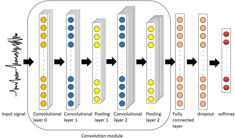
Input layer: The function is to preprocess the original vibration signal in segments, and divide the input signal according to the set time step. The feature extraction layer includes a convolution layer and a pooling layer, which receives vibration data from the input layer, and uses multiple convolution kernels in the convolution layer to extract features from the original vibration signal to obtain multiple feature vectors. The maximum pooling operator reduces the dimension of the feature vector and improves the robustness of nonlinear features. Multiple alternating convolutional pooling layers achieve hierarchical extraction of nonlinear features of input signals. The classification layer consists of two fully-connected layers, of which the first fully-connected layer implements the “flattening” operation on the features, that is, all feature vectors are connected end to end to form a one-dimensional vector. The number of neurons in the second fully connected layer is consistent with the number of fault categories, and the Softmax regression classifier is used to achieve the target output category [15].
One-dimensional convolutional layer: It is composed of several one-dimensional convolution units (convolution kernels), and the parameters of each convolution kernel are obtained by the back propagation algorithm to obtain their optimal values. The purpose of the convolution operation in the convolutional layer is to extract the features of the input samples. The more complex the convolutional network, the more complex the features can be extracted through continuous iterations. Convolution formula:
where: is the input characteristic diagram; is the serial number of the network layer; is the weight parameter; is network offset and is output.
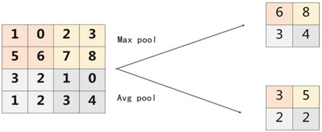
One-dimensional pooling layer: Commonly used are maximum pooling and average pooling. As shown in Fig. 2.
The connection layer: Map the learned “distributed feature representation” to the sample label space.
Classifier: With the “Softmax” classifier, the Softmax classifier is a common linear classifier, which is a generalization of Logistic Regression classifier. The Softmax classifier completes the multi-classification problem. The formula is as follows:
where, represents the output value of the th neuron in the output layer, indicates the output value of the th neuron in the output layer and represents the total number of categories [22].
Fig. 2Schematic diagram of average pooling and maximum pooling
2.2. Principle of learning rate
In machine learning, learning rate is the tuning parameter in the optimization algorithm. Learning rate is an important super parameter in supervised learning and deep learning, and the symbol is , it determines whether and when the objective function can converge to the local minimum. The appropriate learning rate can make the objective function converge to the local minimum in the appropriate time.
However, the selection of learning rate is very difficult, which is determined by the trainers. High learning rate means that the weight update action is larger, so it may take less time to converge to the optimal weight. However, too high a learning rate will lead to too large a beat, which is not accurate enough to reach the best advantage. Since a small learning rate is conducive to the stability of the system, most trainers tend to choose a small learning rate value, which ranges from 0.001 to 0.1 [23].
The value of learning rate is particularly critical to overcome the problem of gradient descent method. An excellent learning rate algorithm can set the appropriate learning rate at different stages of training, so that the model can converge to the optimal solution faster [24]. Too small learning rate will cause slow convergence of the model, and too large learning rate will cause large jitter of the loss function. Therefore, an appropriate learning rate algorithm is very important in the process of depth model training. Table 1 introduces several common learning rate algorithms [25].
Table 1Types of learning rate
Change learning rate | Optimization algorithm |
Fixed attenuation | Piecewise constant attenuation, inverse time attenuation, (natural) exponential attenuation, cosine attenuation |
Periodic change | Cyclic learning rate, SGDR |
self-adaption | Adagrad, RMSporp, AdaDeltea |
3. Experiment and analysis of motor mechanical transmission system
3.1. Experimental test system and data acquisition
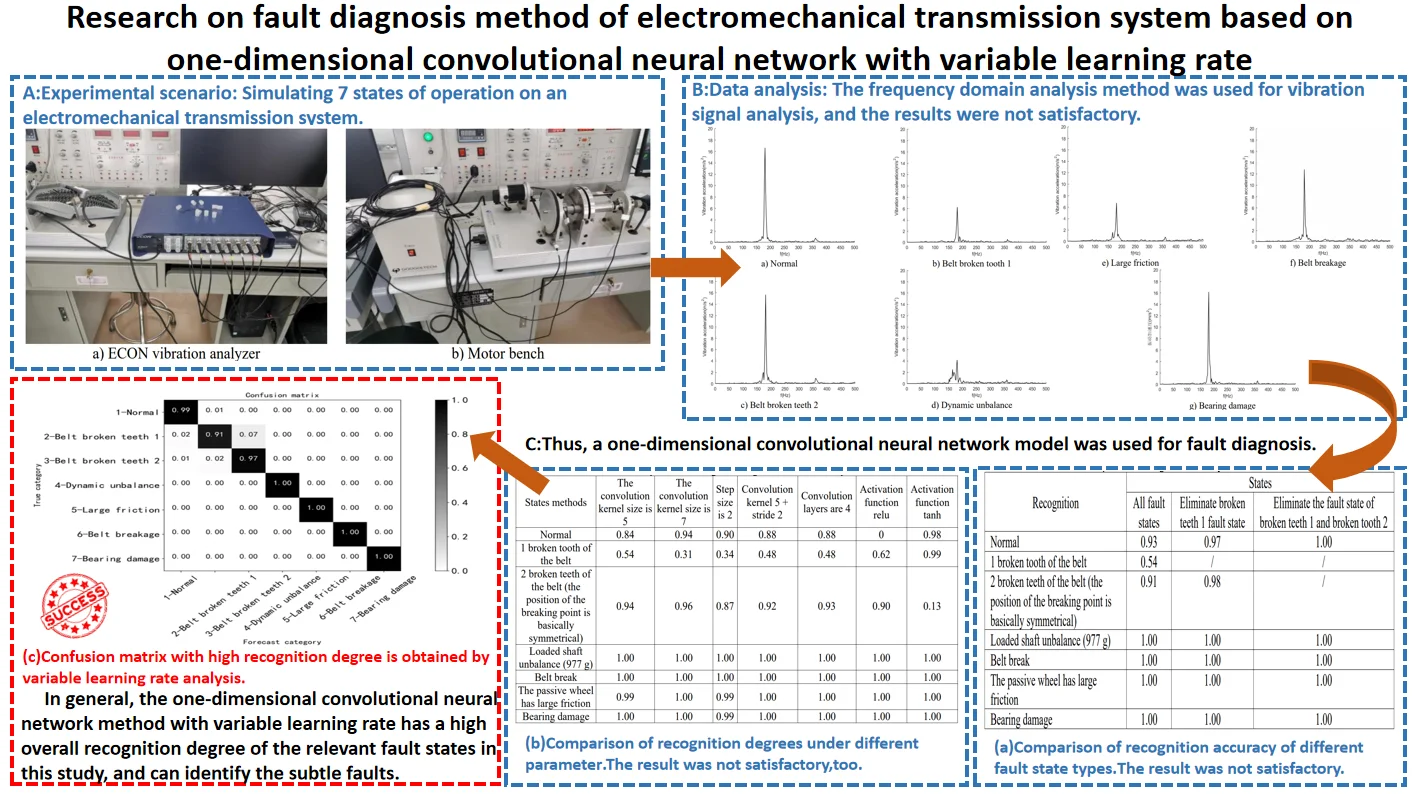
This experimental test system is composed of the experimental platform of DC servo motor system (including the motor bench and Easy Motion Studio software), and ECON acceleration signal acquisition equipment (including ECON vibration analyzer and PC platform), as shown in Fig. 3. Fig. 3 was taken by the author while doing the experiment in the laboratory of Guangdong Polytechnic Normal University. The measured object was a motor bench, and the experimental content included fault setting and vibration acceleration signal acquisition. Three PCB vibration acceleration sensors were pasted on the motor test bench, respectively at the corresponding positions of the rotating shaft and the bearing base.
The experimental protocol is shown in Table 2. Five fault types were set, including one broken tooth of the transmission belt, two broken teeth (the position of the break point is basically symmetric), shaft imbalance, large friction of the passive wheel and bearing damage, etc. Together with the normal state, a total of six state data were analyzed. The detailed working method is as follows: after setting a state, set the speed parameters through Easy Motion Studio software, drived the motor to rotate normally, and use ECON vibration signal acquisition instrument to collect vibration signals. According to the experimental scheme of the motor, each speed was tested three times, about 25 s for each time. The collected signals were named and saved. Then the collected vibration signals are analyzed, including spectrum analysis and one-dimensional convolution neural network analysis.
Fig. 3Test system
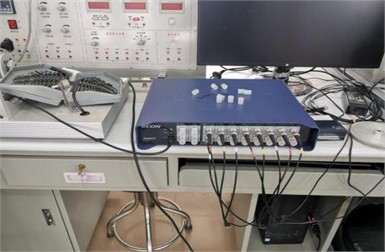
a) ECON vibration analyzer
b) Motor bench
Table 2Experimental scheme of fault setting and data acquisition
No. | Status | Motor speed | Sampling duration |
1 | Normal | 500 rpm 1000 rpm 1500 rpm 2000 rpm 2500 rpm | Each 3 times, each time about 25 s |
2 | 1 broken tooth of the belt, (broken tooth 1 fault state) | ||
2 broken teeth of the belt, and the position of the breaking point is basically symmetrical (broken teeth 2 fault state) | |||
3 | Shaft unbalance (eccentric mass 977 g) | ||
4 | Belt break | ||
5 | The passive wheel has large friction | ||
6 | Bearing damage |
3.2. Vibration signal analysis
Perform spectrum analysis on the collected vibration acceleration signals to understand and observe the dynamic changes and frequency characteristics of different faults, including the main frequency components of the vibration signal, the range of frequency distribution, and the amplitude of each frequency component, so as to obtain information about main frequency values and their corresponding amplitudes that affects the state of the equipment, in order to understand the characteristic information of each fault state of the equipment to a certain extent [26]. The current spectrum analysis is mainly divided into numerical algorithms based on time-domain solution and numerical algorithms based on frequency-domain solution [27]. Among the numerical algorithms based on time-domain solution, the linear acceleration algorithm [28] and Duhamel integral method [29] are the most widely used. The time domain algorithm can be used to determine the dynamic response of the structure under any time-varying external load and initial conditions. Although the time domain algorithm can effectively solve a large number of problems about structural vibration, in some cases, the frequency domain algorithm has more advantages than the time domain algorithm [30-32]. Moreover, due to the introduction of fast Fourier transform (FFT) and other algorithms [33], the operational efficiency of frequency domain algorithms has also been greatly improved. Therefore, frequency domain algorithms have been more and more widely used [34-35]. Therefore, frequency domain analysis is adopted for vibration signal analysis in this experiment.
In this experiment, the normal state of the transmission system, 1 broken tooth of the belt, 2 broken teeth of the belt (the position of the breakpoint is basically symmetrical), shaft unbalance, large friction of the driven wheel, belt break and damage of the bearing were set up. The sampling rate was set to 16384 Hz to collect vibration acceleration signals with sufficient high frequency. Fig. 4 shows the spectrum analysis diagram of vibration acceleration signals in each state at the bearing base position at a speed of 2500 rpm.
It can be seen from Fig. 4 that the overall fluctuation law of the vibration spectrum is similar in the normal state and various fault states. The frequency component corresponding to the maximum amplitude value is about 200 Hz, which corresponds to the meshing frequency between the belt and the output shaft belt wheel. In addition to the main frequency peak, there are also multiple modulation edge bands on both sides of the peak with similar characteristic distributions. It can be seen that the overall law of the spectrum between the normal state and the fault state is similar, and it is difficult to identify specific fault characteristics. Therefore, intelligent diagnosis and recognition can be carried out through the deep learning convolutional neural network method.
Fig. 4Spectrum diagram of vibration acceleration signal
a) Normal
b) Belt broken tooth 1
c) Belt broken teeth 2
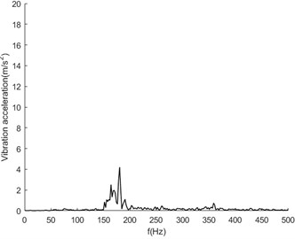
d) Dynamic unbalance
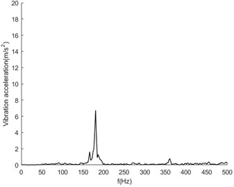
e) Large friction
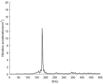
f) Belt breakage
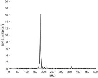
g) Bearing damage
4. Fault classification based on one-dimensional convolutional neural network
In order to effectively reduce the workload of feature extraction and analysis of different state signals, an intelligent diagnosis method based on deep learning is adopted. In this paper, through the 1D-CNN method, in-depth analysis and comparison are carried out for different feature parameters and different network structure parameters, including the size of the convolution kernel, stride, number of convolution layers, activation functions, etc., and obtain a network model with high recognition accuracy.
4.1. Identification analysis for all fault conditions
The 1D-CNN network model is constructed for the data samples under all fault states, and its parameters are shown in Table 3. The input of its one-dimensional convolution neural network is the vibration signal data samples in each state. Through this model, the segmented preprocessing data samples are trained, learned and identified.
Table 31D-CNN model parameters for the full sample size (all fault states)
SN | Step | Layer(type) | Output shape | character |
1 | Input | Input | (None, 400, 9) | |
2 | Convolutional Layer and Pooling Layer | Conv1D | (None, 400, 64) | kernel_size=3, padding = ‘same’ |
3 | LeakyReLU | |||
4 | Conv1D | |||
5 | LeakyReLU | |||
6 | MaxPooling1D | (None, 200, 64) | pool_size=3, strides=2, padding= 'same' | |
7 | Conv1D | (None, 200, 128) | kernel_size=3, padding = ‘same’ | |
8 | LeakyReLU | |||
9 | MaxPooling1D | (None, 100, 128) | pool_size=3, strides=2, padding= ‘same’ | |
10 | Full connected layer | Flatten | (None, 12800) | |
11 | Dense | (None, 128) | ||
12 | LeakyReLU | |||
13 | Dropout | |||
14 | Dense | (None, 32) | ||
15 | LeakyReLU | |||
16 | Dropout | |||
17 | Dense | (None, 7) | ||
18 | LeakyReLU | |||
19 | Output | Softmax | ||
Total params: 1,681,669 Trainable params: 1,681,669 | ||||
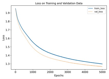
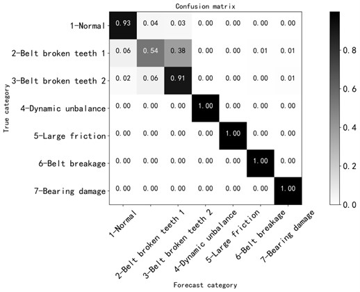
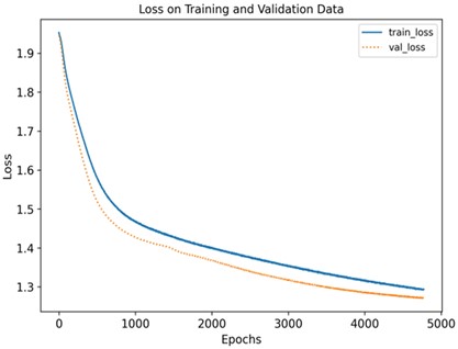
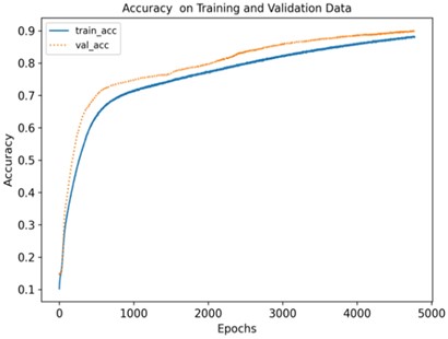
As shown in Fig. 5, it can be seen that after about 5000 iterations, the loss value of the training set and validation set are roughly between 1.35 and 1.4, and the accuracy of the training set and validation set are roughly between 0.8 and 0.9, indicating that the training effect is not ideal. According to the confusion matrix, the recognition degree of each fault type can be known. The recognition degree of the normal state is 0.93, the state of broken tooth 1 is 0.54, the state of broken teeth 2 is 0.91, and the recognition degree of the rest of the fault states is 1, as shown in Fig. 6. The fault states of broken tooth 1 and broken teeth 2 are easy to be confused and difficult to distinguish.
Fig. 5Loss function and accuracy of training and verification
a)
b)
Fig. 6Confusion matrix
4.2. Recognition and analysis under the fault state of removing broken tooth 1
According to the above analysis, the effect of broken tooth fault state is not ideal. The reason is that the broken tooth 1 fault was realized by artificially cutting off one tooth on the inner side of the belt, which is actually a slight fault state, and the vibration response signal of this state is very close to the normal state. Therefore, after removing the fault state of broken tooth 1, the identification analysis is carried out to further grasp the factors affecting the identification accuracy.
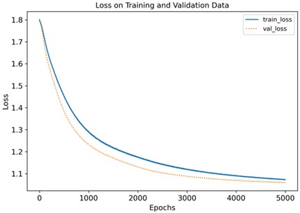
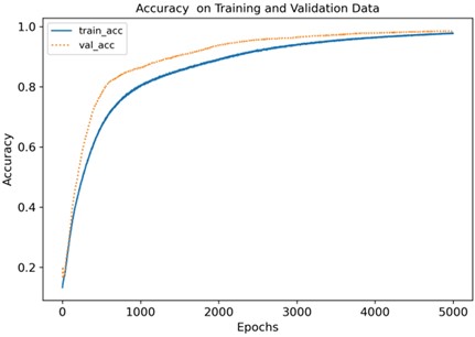
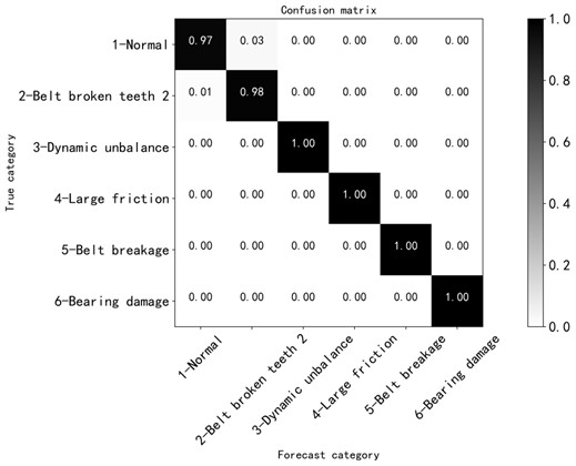
The network structure parameters still use the data in Table 3, and the learning results are shown in Fig. 7. After about 5,000 training iterations, the loss values of the training set and the validation set dropped to between 1.1 and 1.15, the accuracy of the training set and the validation set rose to between 0.9 and 1.0, the accuracy was improved, and the training effect was gradually ideal. It is verified that the fault of broken tooth 1 is similar to the normal state data, and it is indeed difficult to identify, which is consistent with the actual situation. The confusion matrix diagram is shown in Fig. 8. The recognition degree of normal state is 0.97, the recognition degree of broken teeth 2 fault is 0.98, and the recognition degree of other faults is between 1.00, and the recognition degree is greatly improved.
Fig. 7Loss function and accuracy of training and verification
a)
b)
Since the fault degree of broken teeth 2 is also in a slight range, it is also very close to the normal situation. In order to further verify the conclusion, after removing the fault state data of broken teeth 2, the remaining states are trained and learned. After about 3000 training iterations, the loss value of training set and validation set is between 0.9 and 0.95, and the accuracy of training set and validation set is above 0.99. According to the confusion matrix, the recognition degree of each fault is 1.00, and the recognition accuracy is 100 %.
Fig. 8Confusion matrix
4.3. Comparison of identification results under different number of fault states
Based on the above analysis, all the fault state data are trained and tested, and the effect is not ideal. The fault of broken tooth 1 was easily confused with the normal state, and the recognition degree was as low as 0.54. After removing the fault of broken tooth 1 and retraining and testing, the recognition degree has been improved, but the recognition degree is only 0.97 in the normal state, and there is also a recognition error between the fault state of broken teeth 2 and the normal state. After removing all broken tooth fault states, retraining and testing was carried out. It was found that the fault identification degree is improved to 1.00 when the number of training iterations is reduced. The results are shown in Table 4. In general, except for the fault states of broken tooth 1 and broken teeth 2, which are very close to the state data, which are easily confused with the normal state, the network model has high diagnostic and recognition accuracy for the rest of the fault states, and the method is feasible.
Table 4Comparison of recognition accuracy of different fault state types
Recognition | States | ||
All fault states | Eliminate broken teeth 1 fault state | Eliminate the fault state of broken teeth 1 and broken tooth 2 | |
Normal | 0.93 | 0.97 | 1.00 |
1 broken tooth of the belt | 0.54 | / | / |
2 broken teeth of the belt (the position of the breaking point is basically symmetrical) | 0.91 | 0.98 | / |
Loaded shaft unbalance (977 g) | 1.00 | 1.00 | 1.00 |
Belt break | 1.00 | 1.00 | 1.00 |
The passive wheel has large friction | 1.00 | 1.00 | 1.00 |
Bearing damage | 1.00 | 1.00 | 1.00 |
5. Analysis of the influence of different model parameters on the recognition results
After the above analysis, to achieve high-precision identification of 7 fault states, the network parameters shown in Table 3 are not ideal, so we try to adjust the model parameters to find the optimal network structure.
5.1. Different convolution kernel sizes
a) Try to change the size of the convolution kernel from 3 to 5, and verify whether modifying the size parameter of the convolution kernel can improve the recognition degree. After testing, as shown in Fig. 9, it can be seen that after about 5000 iterations, the loss value of the training set and the validation machine is roughly between 1.25 and 1.3, and the accuracy of the training set and the validation set is roughly between 0.85 and 0.9, the confusion matrix in Fig. 10. shows that the recognition degree is 0.54 under the fault state of broken tooth 1 and 0.94 under the fault of broken teeth 2, and the training effect was still not ideal.
Fig. 9Loss function and accuracy of training and verification
a)
b)
b) Continue to try to change the size of the convolution kernel to 7. After training and testing, the following results are obtained: After about 5000 iterations, the loss values of the training set and the validation set are roughly between 1.3 and 1.4, and the loss values of the training set and the validation set are roughly between 1.3 and 1.4. The accuracy of training set and validation set is roughly between 0.85 and 0.9. The training effect is mediocre. It can be seen from the confusion matrix in Fig. 11. that the recognition rate in the fault state of broken tooth 1 is only 0.31, and it was more identified as the fault state of broken teeth 2, which was seriously confused.
Therefore, the size of the convolution kernel is not as large as possible. When the size of the convolution kernel is selected to be 5, the overall recognition degree is relatively high.
Fig. 10Confusion matrix

Fig. 11Confusion matrix
5.2. The case of different sync size
Try to adjust the step size to verify that fault recognition is improved. The original step size is adjusted from 1 to 2. After about 5000 iterations, the loss value of training set and validation set is between 1.3 and 1.4, and the accuracy of training set and validation set is roughly between 0.8 and 0.9. According to the confusion matrix Fig. 12, the recognition rate of broken tooth 1 fault state is 0.34, and 51 % of them are still identified as broken teeth 2 fault, which is not ideal. Moreover, the overall recognition tended to decrease, so the attempt to change the step size did not have the desired effect.
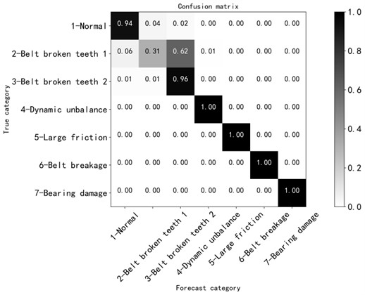
After the above two parameter modifications, the analysis did not get the ideal effect, so we tried to modify the convolution kernel size and step size at the same time for analysis. After about 5000 iterations, the loss values on the training and validation sets are roughly between 1.3 and 1.4, and the accuracy on the training and validation sets are roughly between 0.8 and 0.9. The confusion matrix shows that the recognition degree was 0.88 in the normal state and 0.48 in the fault state of broken tooth 1. The recognition accuracy between the faults of broken tooth 1 and broken teeth 2 was not ideal, especially the fault of broken tooth 1 was identified as the fault of broken teeth 2, as shown in Fig. 13.
Fig. 12Confusion matrix

Fig. 13Confusion matrix

5.3. Different number of convolution layers
Since neither convolution kernel nor step size can be changed to improve fault identification, now we try to increase the number of convolution layers based on convolution kernel of 5 and step size of 2, and increase the original three-layer convolution layer to four-layer convolution layer to verify whether the fault identification can be improved. The confusion matrix is shown in Fig. 14. The recognition accuracy of broken tooth 1 fault is still not significantly improved, and there is no significant difference in the overall state recognition degree. Therefore, the method of increasing the number of convolution layers fails to make the result better.
Fig. 14Confusion matrix
5.4. Use different activation functions
We tried to adjust the activation function to Relu and Tanh functions respectively on the basis of the network structure with convolution kernel size of 5, but the recognition results were not improved for the normal state, broken tooth 1 fault state and broken teeth 2 fault state.
By comparing the recognition accuracy of the above adjusted parameters, it was found that the fault identification degree of the network structure with convolution kernel of 5 was better than that of the network structure with other parameters, as shown in Table 5.
Table 5Comparison of recognition degrees under different parameter
States methods | The convolution kernel size is 5 | The convolution kernel size is 7 | Step size is 2 | Convolution kernel 5 + stride 2 | Convolution layers are 4 | Activation function relu | Activation function tanh |
Normal | 0.84 | 0.94 | 0.90 | 0.88 | 0.88 | 0 | 0.98 |
1 broken tooth of the belt | 0.54 | 0.31 | 0.34 | 0.48 | 0.48 | 0.62 | 0.99 |
2 broken teeth of the belt (the position of the breaking point is basically symmetrical) | 0.94 | 0.96 | 0.87 | 0.92 | 0.93 | 0.90 | 0.13 |
Loaded shaft unbalance (977 g) | 1.00 | 1.00 | 1.00 | 1.00 | 1.00 | 1.00 | 1.00 |
Belt break | 1.00 | 1.00 | 1.00 | 1.00 | 1.00 | 1.00 | 1.00 |
The passive wheel has large friction | 0.99 | 1.00 | 0.99 | 1.00 | 1.00 | 1.00 | 1.00 |
Bearing damage | 1.00 | 1.00 | 0.99 | 1.00 | 1.00 | 1.00 | 1.00 |
5.5. Try VGG11 model
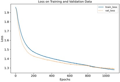
After the above optimization parameters, the desired effect is still not achieved, so we want to optimize the network. The above adjustment is based on one-dimensional convolution neural network. This time, we try to use the classical VGG model. VGG model belongs to the deep convolution neural network model, including VGG11, VGG13, VGG16 and VGG19 models. However, because the VGG11 model has the least number of network layers, less network parameters and low training time cost [36], the VGG11 model is preferred when optimizing the algorithm.
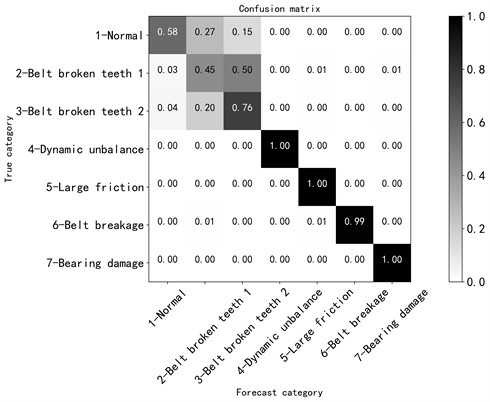
The model is built and tested. It can be seen from Fig. 15 that after about 5000 iterations, the loss value of training set and verification set is about 1.3 to 1.4, and the accuracy rate of training set and verification set is about 0.8 to 0.9. The confusion matrix diagram shows that the recognition degree under normal condition is 0.58, the recognition degree under broken tooth 1 fault condition is 0.45, and the recognition degree under broken tooth 2 fault condition is 0.76, as shown in Fig. 16. None of them is ideal, and there is no obvious improvement compared with one-dimensional convolution neural network, as shown in Table 6.
Fig. 15Loss function and accuracy of training and verification
a)
b)
Table 6Model comparison
Recognition | States | |
One-dimensional convolution neural network | VGG11 model | |
Normal | 0.93 | 0.58 |
1 broken tooth of the belt | 0.54 | 0.45 |
2 broken teeth of the belt (the position of the breaking point is basically symmetrical) | 0.91 | 0.86 |
Loaded shaft unbalance (977 g) | 1.00 | 1.00 |
Belt break | 1.00 | 1.00 |
The passive wheel has large friction | 1.00 | 0.99 |
Bearing damage | 1.00 | 1.00 |
Fig. 16Confusion matrix
5.6. Summary of parameter selection
According to the characteristics of samples, the basic structure of the classical model VGG was adapted to construct a one-dimensional convolutional neural network. Since the recognition is still not ideal when the convolution kernel is 3, attempts are made to expand the convolution kernel, increase the global attention of the convolution kernel, capture global features, and then conduct training. Since it is verified that the means of expanding convolution kernel has no obvious effect on the improvement of fault recognition degree, the small verification step size has an impact on the recognition degree. Adjusting the convolution kernel size can reduce the number of sample parameters after convolution, reduce the sample complexity and improve the training rate. It has been verified above that changing the size of convolution kernel and changing the size of step cannot improve the recognition, so try to change the number of convolution layers. Generally speaking, changing the number of convolutional layers can change the depth of the network, making the training more efficient and affecting the accuracy of recognition. Different activation functions can change the linear fitting ability and learning efficiency of the model. However, in the case of small and similar fault states, all the states cannot be well identified by the above method of parameter adjustment. Try again to optimize the network model, try VGG11 model, but the ideal effect is not achieved.
6. Analysis of the results of the variable learning rate method
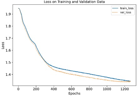
After adjusting the parameters for several times, the failure of this experiment could not be solved successfully. After consulting relevant literature, it was found that adjusting the learning rate could better train the network. Variable learning rate means that different learning rates are adopted in different learning stages, so that the objective function reaches the local optimal solution at different rates in different stages. It can improve the learning rate and change the result under the condition of the same learning times (epoch). Meanwhile, in the process of analysis, it is found that the recognition accuracy can be relatively improved by changing the learning rate on the basis of the convolution kernel being 5, so the learning rate is analyzed at a deeper level. In the network structure with convolution kernel of 5, through debugging and analysis, it was found that the test result with learning rate of 0.9e-6 was relatively good, and with debugging learning rate of 5e-6, the accuracy of the first 800 epochs can reach about 80 %, as shown in Fig. 17(a). Therefore, in the learning process, the variable learning rate method was adopted to continue the training and learning to obtain a better fault recognition rate.
Fig. 17Loss function and accuracy of training and verification with a learning rate of 5e-6
a)
b)
Fig. 18Loss function and accuracy of training and verification under two learning rates
a)
b)
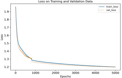
For the same number of learning steps, two different learning rates are adopted for training. The learning rate of the first 800 epochs is set as 5e-6, and the learning rate of the last 4200 epochs is set as 0.9e-6. After testing, the results shown in Fig. 17(b) are obtained.
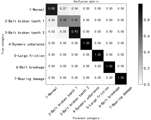
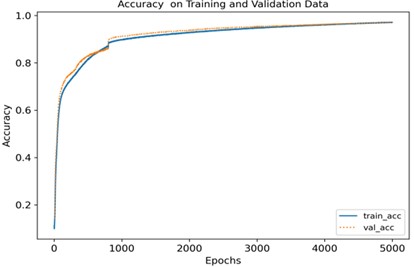
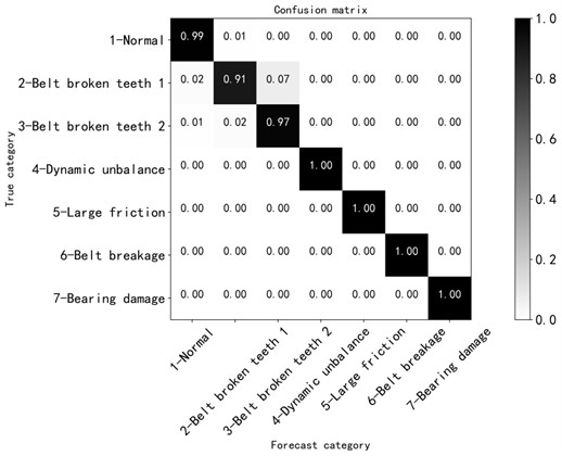
It can be seen from Fig. 18 that after about 5000 iterations, the loss values of the training set and the validation set are roughly between 1.2 and 1.3, and the accuracy was between 0.9 and 1.0, and the training effect is better. According to the confusion matrix in Fig. 19, the recognition degree of each fault is above 0.9, the recognition degree of the normal state is 0.99, the recognition degree of the broken tooth 1 fault state and the broken teeth 2 fault state are 0.91 and 0.97 respectively, compared with the method of adjustment in front of the other parameters, the accuracy is improved, and the recognition degree of other fault states is 1.00, which is ideal.
In general, the one-dimensional convolutional neural network method with variable learning rate has a high overall recognition degree of the relevant fault states in this study, and can identify the subtle faults such as broken teeth 1 and broken tooth 2.
Fig. 19Confusion matrix
7. Conclusions
In the motor mechanical transmission system, the vibration acceleration signal data of various fault states of the motor were collected, and the one-dimensional convolutional neural network model in the deep learning method was used for diagnosis analysis and research. By adjusting different network structure parameters and making comparative analysis, it is found that the method of changing the learning rate has higher recognition accuracy in all fault states (including slightly similar states). The analysis results show that the fault diagnosis of electromechanical transmission system using 1D-CNN analysis method is easier to identify the fault state intelligently than the pure vibration signal spectrum analysis method, and this research enriches the diagnosis experience of electromechanical transmission subtle faults, which is a novel contribution. At the same time, it can also provide good guidance for the real-time monitoring application of other types of transmission systems.
References
-
S. Ding et al., “Research status and prospect of deep learning theory and its application in motor fault diagnosis,” Power System Protection and Control, Vol. 48, No. 8, pp. 172–187, 2020, https://doi.org/10.19783/j.cnki.pspc.190712
-
D. Liu, “Application of deep learning in bearing fault diagnosis,” Science and Technology Wind, No. 9, pp. 91–93, 2022, https://doi.org/10.19392/j.cnki.1671-7341.202209031
-
Q. Yao et al., “Application of Deep learning in modern medical field,” Application of Computer Systems, Vol. 31, No. 4, pp. 33–46, 2022.
-
Indrajani Sutedja, “Descriptive and predictive analysis on heart disease with machine learning and deep learning,” in 3rd International Conference on Cybernetics and Intelligent System (ICORIS), pp. 1–6, 2021.
-
Amani Yahyaoui and N. Yumusak, “Deep and machine learning towards pneumonia and asthma detection,” in International Conference on Innovation and Intelligence for Informatics, Computing, and Technologies (3ICT), pp. 494–497, 2021.
-
Rao Kunal, Gopal Pawan-Raj, and Lata Kusum, “Computational analysis of machine learning algorithms to predict heart disease,” in 11th International Conference on Cloud Computing, Data Science and Engineering, pp. 960–964, 2021.
-
Shi Dong, Yuanjun Xia, and Tao Peng, “Network abnormal traffic detection model based on semi-supervised deep reinforcement learning,” IEEE Transactions on Network and Service Management, Vol. 18, No. 4, pp. 4197–4212, 2021.
-
C. Ma, “Application analysis of deep learning in motor fault diagnosis,” Power Equipment Management, Vol. 6, pp. 193–195, 2021.
-
Y. Long and H. He, “Robot path planning based on deep reinforcement learning,” in IEEE Conference on Telecommunications, Optics and Computer Science, pp. 151–154, 2020.
-
N. F. Mir, A. S. H. Basha, and A. A. K. Tiwari, “Application of deep learning in dynamic link-level virtualization of cloud networks through the learning process,” in 2021 International Symposium on Computer Science and Intelligent Controls (ISCSIC), pp. 169–173, Nov. 2021, https://doi.org/10.1109/iscsic54682.2021.00040
-
W. Deng, J. Xu, X.-Z. Gao, and H. Zhao, “An enhanced MSIQDE algorithm with novel multiple strategies for global optimization problems,” IEEE Transactions on Systems, Man, and Cybernetics: Systems, Vol. 52, No. 3, pp. 1578–1587, Mar. 2022, https://doi.org/10.1109/tsmc.2020.3030792
-
H. Zhao et al., “Intelligent diagnosis using continuous wavelet transform and gauss convolutional deep belief network,” IEEE Transactions on Reliability, pp. 1–11, 2022, https://doi.org/10.1109/tr.2022.3180273
-
W. Deng et al., “Multi-strategy particle swarm and ant colony hybrid optimization for airport taxiway planning problem,” Information Sciences, Vol. 612, pp. 576–593, Oct. 2022, https://doi.org/10.1016/j.ins.2022.08.115
-
K. Liu et al., “Target classification of aerial reconnaissance and forensics based on deep learning,” (in Chinese), Ordnance Industry Automation, Vol. 41, No. 4, pp. 60–63, 2022.
-
S. Chen et al., “A fault diagnosis method of hydraulic system based on 1DCNN and multi-sensor information fusion,” (in Chinese), Mechanical Science and Technology, No. 9, pp. 1–9, 2022, https://doi.org/10.13433/j.cnki.1003-8728.20220028
-
M. Wang, “Bearing fault diagnosis method based on variable learning rate multilayer perceptron,” (in Chinese), Science and Technology Information, Vol. 20, No. 8, pp. 52–55, 2022, https://doi.org/10.16661/j.cnki.1672-3791.2201-5042-6538
-
S. Chen, G. Wang, and D. Zhang, “Research on fault prediction of wind turbine based on improved variable learning rate neural network,” (in Chinese), Heilongjiang Electric Power, Vol. 43, No. 2, pp. 99–102, 2021, https://doi.org/10.13625/j.cnki.hljep.2021.02.002
-
C. He and B. Yin, “Research on autonomous navigation of deep-sea autonomous robot (AUV) – variable learning rate online optimization algorithm,” (in Chinese), China Engineering Consulting, Vol. 172, No. 1, pp. 47–50, 2015.
-
Canyi Du et al., “UAV rotor fault diagnosis based on interval sampling reconstruction of vibration signals and a 1D-CNN deep learning method,” Measurement Science and Technology, Vol. 33, No. 6, 2022.
-
Q. Chu et al., “Gear fault diagnosis based on multifractal theory and neural network,” (in Chinese), Vibration and Shock, Vol. 34, No. 21, pp. 15–18, 2015, https://doi.org/10.13465/j.cnki.jvs.2015.21.003
-
J. Qu et al., “Adaptive fault diagnosis algorithm for rolling bearings based on one-dimensional convolutional neural networks,” Journal of Instrumentation, Vol. 39, No. 7, pp. 134–143, 2018, https://doi.org/10.19650/j.cnki.cjsi.j1803286
-
D. H. Hubel and T. N. Wiesel, “Receptive fields, binocular interaction and functional architecture in the cat's visual cortex,” The Journal of Physiology, Vol. 160, No. 1, pp. 106–154, Jan. 1962, https://doi.org/10.1113/jphysiol.1962.sp006837
-
B. L. Y. He, “A combined deep learning model learning rate strategy,” Journal of Automation, Vol. 42, No. 6, pp. 953–958, 2016, https://doi.org/10.16383/j.aas.2016.c150681
-
Kazuma Itakura, Kyohei Atarashi, S. Oyama, and M. Kurihara, “Adapting the learning rate of the learning rate in hypergradient descent,” 2020 Joint 11th International Conference on Soft Computing and Intelligent Systems and 21st International Symposium on Advanced Intelligent Systems (SCIS-ISIS), 2020.
-
H. Lin, “Research on learning rate algorithm in deep neural network training,” Zhejiang Business University, Lin Hong, 2022.
-
J. Wang and F. Li, “Signal processing method for mechanical fault diagnosis: frequency domain analysis,” (in Chinese), Noise and Vibration Control, Vol. 33, No. 1, pp. 173–180, 2013, https://doi.org/10.27462/d.cnki.ghzhc.2022.000757
-
R. Clough, J. Penzien, and D. Griffin, Dynamics of Structures. New York: McGraw-Hill, 1975.
-
N. M. Newmark, “A Method of Computation for Structural Dynamics,” Journal of the Engineering Mechanics Division, Vol. 85, No. 3, pp. 67–94, 1959.
-
A. K. Chopra, Dynamics of Structures. New York: Pearson Education Inc, 2007.
-
L. Deng et al., “Analysis on frequency response of floating wind turbine considering the influence of aerodynamic damping,” (in Chinese), Journal of Hunan University (Natural Sciences), Vol. 31, No. 3, pp. 68–71, 2004, https://doi.org/10.16339/j.cnki.hdxbzkb.2017.01.001
-
W. Yi, W. Ma, and G. Liu, “Modal analysis of soil-structure dynamic interaction,” (in Chinese), Journal of Hunan University (Natural Science), Vol. 31, No. 3, pp. 68–71, 2004.
-
L. Li, Y. Hu, and X. Wang, “Improved approximate methods for calculating frequency response function matrix and response of MDOF systems with viscoelastic hereditary terms,” Journal of Sound and Vibration, Vol. 332, No. 15, pp. 3945–3956, Jul. 2013, https://doi.org/10.1016/j.jsv.2013.01.043
-
J. W. Cooley and J. W. Tukey, “An algorithm for the machine calculation of complex Fourier series,” Mathematics of Computation, Vol. 19, No. 90, pp. 297–301, Jan. 1965, https://doi.org/10.1090/s0025-5718-1965-0178586-1
-
X. Han, W. Qiao, and B. Zhou, “Frequency domain response of jacket platforms under random wave loads,” Journal of Marine Science and Engineering, Vol. 7, No. 10, p. 328, Sep. 2019, https://doi.org/10.3390/jmse7100328
-
F. Lemmer, W. Yu, and P. Cheng, “Iterative frequency-domain response of floating offshore wind turbines with parametric drag,” Journal of Marine Science and Engineering, Vol. 6, No. 4, p. 118, Oct. 2018, https://doi.org/10.3390/jmse6040118
-
L. Liao, S. Li, and X. Wang, “Photolithography bad point detection method based on pre-training VGG11 model,” (in Chinese), Journal of Optics, pp. 1–18, 2023.
About this article

The authors have not disclosed any funding.
The datasets generated during and/or analyzed during the current study are available from the corresponding author on reasonable request.
Liwu Liu’s contributor role are methodology, data curation and software. Guoyan Chen’s contributor role are methodology, writing – original draft preparation and writing–review and editing. Feifei Yu’s contributor role are project administration and resources. Canyi Du’s contributor role are supervision, conceptualization and writing-review and editing. Yongkang Gong’s contributor role are supervision and resources. Huijin Yuan’s contributor role are investigation and validation. Zhenni Dai’s contributor role are investigation and validation.
The authors declare that they have no conflict of interest.
