Abstract
In order to solve the dependence of convolutional neural networks (CNN) on large samples of training data, an intelligent fault diagnosis method based on spectral kurtosis (SK) and attention mechanism is proposed. Firstly, the SK algorithm is used to obtain two-dimensional fast kurtosis graphs from vibration signals, and the two-dimensional fast spectral kurtosis graphs are converted into one-dimensional kurtosis time-domain samples, which are used as the input of CNN. Then the channel attention module (CAM) is added to CNN, and the weight is increased in the channel domain to eliminate the interference of invalid features. The accuracy of fault identification can reach 99.8 % by applying the proposed method on the fault diagnosis experiment of rolling bearings. Compared with the traditional deep learning (DL) method, the proposed method not only has higher accuracy, but also has lower dependence on the number of samples.
1. Introduction
Because of the rolling bearing’s long-term operation and poor working environment, it is easy to damage its internal structure, which leads to equipment failure and causes economic losses and even casualties [1-2]. Therefore, reliable fault diagnosis technology becomes the key to real-time detection of equipment health status.
In the data mining algorithm, CNN has been used widely because of its powerful local feature learning ability and flexible structure, and successfully applied in the fault diagnosis field [3-4]. A diagnostic model combining continuous wavelet transform with binary CNN is proposed [5], which replaces the traditional convolution layer with binary convolution, so that the model has a faster training speed. The residual learning module is embedded into CNN to increase the depth of the network model and prevent overfitting [6]. A multi-channel CNN (MCNN) [7] diagnosis model was proposed: Multi-scale fusion (MSCF) and STFT were used for data preprocessing, and MCNN was used for fault classification. Wang et al proposed a multi-task CNN(MACNN) [8], and introduced Atlas convolutional layer module and parallel multiple independent output layer to enhance feature learning ability. Wang et al [9] solved the sparse coefficient by using OMP algorithm, in which the fault features were represented sparsely, and the reconstructed fault feature signals were obtained and input into CNN for fault diagnosis. Shao et al [10] proposed a diagnosis method based on 1DCNN and INS0-SVM: 1DCNN was used to extract fault features, and the extracted features were used for SVM training to classify faults. Jin et al [11] proposed a light neural network to reduce CNN parameters, so as to accelerate fault identification and improve fault diagnosis efficiency. A Fault diagnosis method for material handling system using feature selection and data mining techniques is proposed in [12].
Although the intelligent diagnosis method based on CNN has been successfully applied in the field of fault diagnosis, there are still some problems to be solved:
(1) In actual working conditions, the features of faulty bearing are usually interfered by noise and other characteristic information. Many fault diagnosis methods based on CNN set aside the knowledge of diagnosis domain, resulting in poor diagnosis effect.
(2) The excellent feature learning ability of CNN depends on a large number of data sets. However, in actual working conditions, the amount of fault data collected is usually limited. When smaller data sets are used, network degradation may occur in the model due to excessive CNN network parameters.
According to the above problems, the rolling bearing fault mechanism is fully introduced into the data preprocessing stage, and the knowledge in the field of kurtosis is introduced. Kurtosis is a dimensionless index in time domain, which is sensitive to the transient impact component buried in the signal [13], but it is easily disturbed by noise, resulting in poor effect. Spectral kurtosis was proposed by Deyer [14] to identify transient impact components from background noise by calculating the higher-order statistics of each spectral line kurtosis. Wan et al [15] improved the maximum correlation kurtosis deconvolution (MCKD) to extract composite fault information in different frequency bands. After MCKD processing, Fast spectral kurtosis (FSK) analysis was used to further identify the resonant frequency. Jing et al [16] used EMD data preprocessing to obtain the reconstructed signal, and then designed a suitable filter to filter the reconstructed signal through FSK to eliminate interferences, and finally analyzed the envelope demodulation result for feature extraction. Inspired by the aforementioned literatures, the SK algorithm is used to obtain the high-order statistics of each spectral line kurtosis in the vibration signal, and takes them as the input of CNN to enhance the feature representation. The important contributions of this paper are as following: (1) A fault diagnosis method based on SK feature extraction and CAM-CNN is proposed to solve the dependence of CNN on large data sets. (2) This method uses SK for preprocessing to enhance feature representation and reduce the learning difficulty of CNN. (3) CAM modules are embedded in CNN to distinguish the importance of each channel and improve the efficiency and accuracy of the network model.
2. Spectral kurtosis
Antoni [17] proposed a FIR - based FSK algorithm, and its basic principle is to decompose the original signal with a 1/3- binary tree filter, and then calculate the kurtosis value of each frequency of the decomposed signal. The specific method is to select a suitable high-pass filter and low-pass filter , as shown in Fig. 1, the specific formula is as following:
among them, is the FIR low-pass filter, and the cut-off frequency is .
Fig. 1Decomposition of high-pass filter and low-pass filter
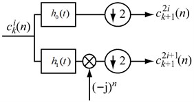
and are used to filter the analyzed signal respectively, and the filtering results are sampled twice down. In this way, the corresponding filtering results are obtained iteratively. The filtering results include the filtered results of center frequency and bandwidth, and the spectral kurtosis is calculated according to Eq. (2):
Finally, all the calculated spectral kurtosis are integrated to form the fast spectral kurtosis graph of signal .
3. Channel attention mechanism
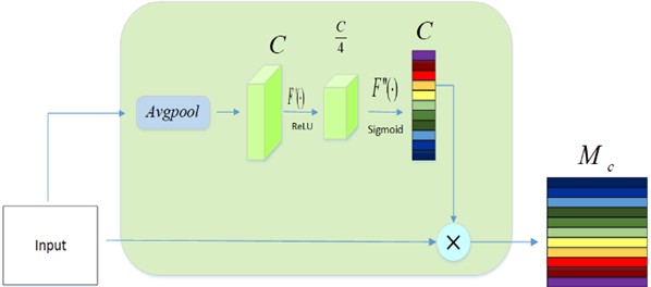
Because some feature information may have nothing to do with fault location, and different convolutional checks have different recognition degrees of feature information, which may result in judgment errors [18]. The channel attention mechanism weights each feature channel to enhance effective features and suppress redundant information, so as to eliminate the interference of noise and other invalid features adaptively [19].
The basic structure diagram of CAM is shown in Fig. 2. CAM weights each characteristic channel through modeling, and then enhances or suppresses different feature channels for different tasks. The input is a combination of channel . First, the feature map of each channel is compressed to a single value of by using the GAP. Calculate the th according to the following formula:
Embed two dimensions of information into . A set of weights are learned with two fully connected layers after dimension reduction and dimension increasing, and channel weight feature is generated, which is defined as follows:
where, represents the RELU activation function. drop the number of channels through the first full collection layer (FC), and recovers the original number of channels through the second FC, which encode channel correlation. is the Sigmoid function, and the weight of the encoded channel is normalized to between 0 and 1, so as to obtain the weight value of each channel . represents the weight of the whole channel. Multiply the normalized weight feature with the input:
Fig. 2Feature enhancement module based on channel mechanism
4. CNN
CNN is mainly composed of convolution layer, pooling layer and full connection layer (FC). Its structure is shown in Fig. 3. The convolutional layer is mainly used for feature extraction, the pooling layer mainly reduces the dimension and fewer network parameters, and FC classifies the extracted features.
Fig. 3Classical architecture of convolutional neural network
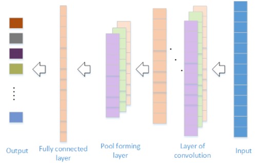
4.1. Convolution layer
The convolution layer generates specific feature sequences by performing local convolution operations on inputs, and different convolution kernels learn the weights of different regions of the original signal. Eq. (6) is convolution operation:
where, is the th weight learned from the rd convolution layer, is the 5 convoluted part local region of the convolution in layer , and is the size of the convolution kernel.
4.2. Pooling layer
The sequence of features increases after convolving the input, which results in an increase in dimension. Pooling layer prevents overfitting by reducing data to reduce network parameters. Pooling function mainly includes average pooling and maximum pooling. Maximum pooling is adopted in this paper, and its formula is as follows:
where, is an element of the convolution core in the convolution layer, is the size of the target area, and is the output of the maximum pooling function.
4.3. Full Connection layer
The FC classifies the features learned from the convolution kernel, and reduces the dimensions of the features learned from the convolution core. Besides, FC also updates and reorganizes the weights. The formula of FC is as follows:
where, is the weight between convolution cores in different convolution layers. is the pair value of the th output convolution kernel in layer . is the shift of the convolution core in the convolution layer relative to the convolution core in the next convolution layer.
5. Construction of SK-CAM-CNN model
In practical engineering, the impact incomplete period is caused by the instability of velocity, the change of load and the random deviation of rolling elements. In this case, the traditional time fault diagnosis method usually could not extract the fault information perfectly under the interference of background noise. To this end, SK is introduced to preprocess the data, and the data set is obtained by using the data enhancement technology with fixed length random segmentation. Then the kurtosis value is calculated, and the unique characteristic signal is extracted. Finally, CNN is used for fault classification and diagnosis.
5.1. Convolutional neural network based on CAM
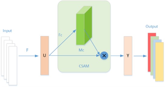
In order to enhance the adaptive ability of the convolution check receptive field size and improve the recognition ability of the network model to fault features, a CAM-based multi-layer convolutional network is proposed. Its structure is shown in Fig. 4.
For input , the initial feature extraction is completed by the first layer of wide convolution, and the input feature elements are compressed () in operation , which is mainly completed by global average pooling (GAP). In operation of , the compressed feature elements are mainly integrated into the fully connected layer to predict the importance of each channel, and then the obtained weights are multiplied by the features of the upper layer to realize the weighting of channels. Then it is input to the next layer of convolution to complete the final feature extraction, and the learned features are classified to get the output results.
Fig. 4Convolutional neural network based on channel attention mechanism
5.2. Fault diagnosis framework based on SK and CNN
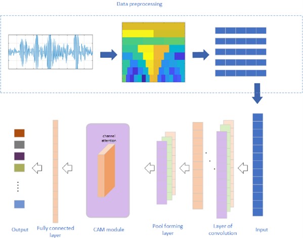
The combination of spectral kurtosis preprocessing with CAM-CNN was applied on bearing fault diagnosis. Firstly, the collected vibration signal is preprocessed in the kurtosis domain to obtain the kurtosis map, and then transform the two-dimensional kurtosis map into one-dimensional kurtosis time domain samples. Then, one-dimensional time-domain kurtosis samples are input into CNN for training, and the network introduces CAM module to update the weight, which further improves the feature learning ability of the network. The entire diagnostic process is shown in Fig. 5.
Step 1: First, one-dimensional vibration signals are collected, and the fixed-length random segmentation data enhancement technology is adopted to obtain training and test data.
Step 2: Perform spectral kurtosis analysis on the enhanced data, and the obtained fast spectral kurtosis graph is transformed into a one-dimensional kurtosis time domain sample, which is used as input of CNN.
Step 3: After the convolution, BN and pooling operations, the features learned from the convolution kernel are input into the CAM module, and the network channel weights are updated to eliminate the interference of invalid features.
Step 4: Use the training set training model and optimize the network parameters by Adam algorithm. A network model based on SK-CAM-CNN is established.
Step 5: Input the test set into the CAM-CNN model to obtain visual results.
Fig. 5Flow chart of convolutional neural network based on spectral kurtosis feature extraction and channel attention mechanism
6. Verification by experiment 1
6.1. Data description
The validity of the proposed model is verified by the rolling bearing data set of Western Reserve University. Fig. 6 shows the rolling bearing test platform. In addition to normal state (NC), SKF deep groove ball bearings also introduce three kinds of faults, namely inner ring fault (IF), outer ring fault (OFS) and rolling body fault (BFS). There are three fault types of faulty bearings, with fault diameters of 0.1778 mm, 0.3556 mm and 0.5334 mm respectively. There are 7 bearing health states (NC, BF14, BF21, IF7, IF14, OR7, OR14) corresponding to the shaft speed of 1772 r/min under 1 HP load. Fig. 7 shows the three-dimensional time-domain waveform of rolling bearings under three different loads.
In this test, the minimum bearing speed was 1772 r/min. In order to fully ensure the integrity and reliability of fault information of each data sample, the length of each data sample was set as 1024 sampling points, and the fixed-length random segmentation data enhancement technology was adopted to obtain training and test data. Sample data of 7 original one-dimensional vibration signals are labeled. Each type of signal contains 200 samples, a total of 1400 samples, which are divided into training set, test set and verification set with ratio of 7:2:1. The distribution of bearing fault samples is shown in Table 1.
Fig. 6Rolling shaft data acquisition experimental bench
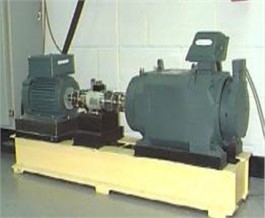
Fig. 7Time domain waveforms of different fault signals under three loads
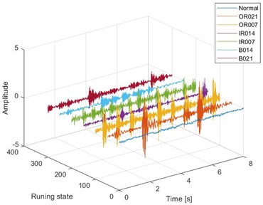
a) 1 HP

b) 2 HP
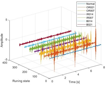
c)
6.2. Setting of CNN structure
Construct CNN based on CAM. The CNN architecture consists of five layers of convolution layer, five layers of pooling layer, CAM module, full connection layer and Soft-max layer. The CAM module is set after the first layer of pooling and before the second layer of convolution. The step size of the convolution layer is set as 1, and the number of convolution kernels of the first convolution layer is set as 16. The latter layer has twice as many convolution kernels as the previous one. Zero convolution padding is used to preserve the size of the space between the input and output volumes. Pooling layer adopts maximum pooling and window span is 2. The last layer is Soft-max layer, and the model parameters are shown in Table 2.
Table 1Distribution of rolling bearing fault samples
Diameter of failure / mm | 0 | 0.1778 | 0.3556 | 0.5334 | Load / HP | |||||
Normal | Inner ring | Outer ring | Body of rolling | Outer ring | Inner ring | Body of rolling | ||||
Fault label | 0 | 1 | 2 | 3 | 4 | 5 | 6 | |||
A | Set of training | 700 | 700 | 700 | 700 | 700 | 700 | 700 | 1 | |
Set of tests | 200 | 200 | 200 | 200 | 200 | 200 | 200 | |||
Set of verification | 100 | 100 | 100 | 100 | 100 | 100 | 100 | |||
B | Set of training | 700 | 700 | 700 | 700 | 700 | 700 | 700 | 2 | |
Set of tests | 200 | 200 | 200 | 200 | 200 | 200 | 200 | |||
Set of verification | 100 | 100 | 100 | 100 | 100 | 100 | 100 | |||
C | Set of training | 700 | 700 | 700 | 700 | 700 | 700 | 700 | 3 | |
Set of tests | 200 | 200 | 200 | 200 | 200 | 200 | 200 | |||
Set of verification | 100 | 100 | 100 | 100 | 100 | 100 | 100 | |||
Table 2CAM-CNN model parameters
Layer | Layer type | Kernel | Number of filters | Filter size | Output Size |
1 | Input | / | / | / | (1024,1) |
2 | Conv | Kernels | 16 | 64*1 | (128,16) |
4 | Glob | / | / | / | (16) |
5 | FC | / | / | 68 | (4,1) |
6 | ReLU | / | / | / | (4,1) |
7 | FC | / | / | 80 | (16,1) |
8 | Multiply | / | / | / | (128,16) |
11 | Conv1D | Kernels | 1 | (128,16) | |
13 | conv1d_2 | Kernels | / | / | (64,32) |
14 | conv1d_3 | Kernels | / | / | (32,64) |
15 | conv1d_4 | Kernels | / | / | (16,128) |
16 | conv1d_5 | Kernels | / | / | (16,256) |
17 | Dropout | Dropout rate | / | 0.5 | (16,256) |
18 | Fc | / | / | 42 | (16,1) |
6.3. Analysis and discussion
6.3.1. Analysis of experimental results
The data set with load of 1HP was selected for testing. After 100 rounds of training, the model got the test results as shown in Fig. 8, which showed that the diagnostic accuracy could reach 99.92 %. The loss curve leveled off after 20 rounds of training. Therefore, it is verified that SK-CAM-CNN has high accuracy in rolling bearing fault diagnosis.
The confusion matrix represents the type and number of misjudgments under different fault types. The confusion matrix is used to further verify the fault recognition ability of the model. The experimental results shown in Fig. 9: 1400 test samples are all correctly identified, which further verified the excellent fault recognition capability of the proposed model.
In order to show the ability of fault identification more intuitively, the classification results of deep neural network are clearly displayed by using t-SNE visualization technology. Ten kinds of bearing data diagnosis processes with motor loads of 1 HP, 2 HP and 3 HP are selected for visualization, and the experimental results are shown in Fig. 10. The original data is processed by the proposed method, and all data features are obviously classified and clustered. It can be found that the model can correctly classify 10 fault features, which shows that the model has good diagnostic performance.
Fig. 8Accuracy and loss curves of the model after training
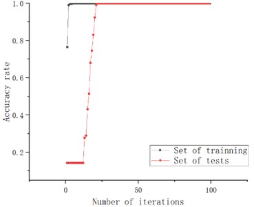
a) Accuracy with number of iterations
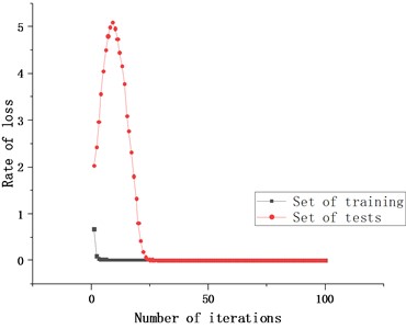
b) Loss with number of iterations
Fig. 9Confusion matrix of rolling bearing classification
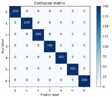
Fig. 10visualization results of t-SNE under three different loads
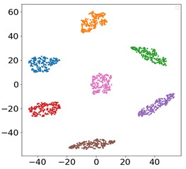
a) 1 HP
b) 2 HP
c) 3 HP
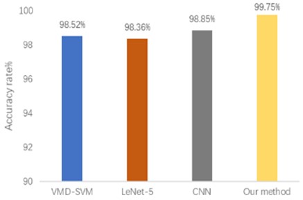
In this paper, EMD-SVM [20] based on artificial filtering, CNN [21] based on DL and Lenet-5 [22] are selected for comparison. 10 experiments are carried out with 1HP data set, and the average accuracy was taken 10 times. The results are shown in Fig. 11. The fault identification accuracy of this method is higher than that of the other three methods. Experimental results verify the effectiveness of SK pretreatment and CAM module.
Fig. 11Diagnostic accuracy of different models
6.3.2. Performance analysis of the model under different data set sizes
The amount of collected fault data is usually limited in actual operating conditions. When smaller data sets are used, network degradation may occur in the model with the depth of the deep learning network increasing. Therefore, it is very important for the fault diagnosis model to have a good diagnostic effect under smaller samples. This paper conducts experiments on the data of 1 HP, and compares and analyzes the data under five different scales of 100 %, 80 %, 60 %, 40 % and 20 % of the total data set, and conducts 20 tests on the reduced data set and then averages the results, and the results were shown in Fig. 11.
Fig. 12Accuracy for different data set sizes
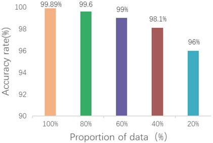
As can be seen from the diagnostic results in the Fig. 12, the proposed model has a high accuracy in different scale data sets except that the diagnostic effect decreases in 20 % case. Therefore, it still has good accuracy and stability under small scale data set.
6.3.3. Generalized performance analysis of the model under different load conditions
The load of rolling bearings often changes under the influence of working environment, so it is very important to maintain good diagnostic effect under different load conditions. Three data sets under different loads were tested to verify the diagnostic performance of the model under different loads. Data sets A, B, and C represent data at 1, 2, and 3 horsepower loads, respectively. Taking A→B as an example, data set A is used to train the network model, and data set B is used to test the network model. The experimental results averaged 20 times.
Data sets under three different loads are tested and compared with EMD-SVM, CNN and Lenet-5 methods. Table 3 shows the fault diagnosis results of the four methods under different loads. Experimental results show that the diagnostic effect of this method is better than the other three methods under different loads. Taking C→A and C→B as examples, the fault recognition accuracy of VMD-SVM based on feature extraction is only 85.69 % in different load domains due to the problem of modal confusion. CNN and LeNet-5 based on DL model use two-dimensional data as network input. The conversion of one-dimensional data to two-dimensional data may result in the loss of fault characteristic information. Therefore, the fault diagnosis rates of these two methods are only 94.76 % and 94.36 % under different loads. In the C→A and C→B experiments under different loads, the fault diagnosis rate of the proposed method is above 97 %, and the average accuracy of all experiments under different loads is 98.33 %. This is because the diagnosis domain knowledge is introduced before diagnosis, and spectral kurtosis preprocessing is carried out to enhance the fault mode of each category, thus reducing the difficulty of learning CNN. At the same time, the CAM module is added to CNN to extract the beneficial features of the network model in a weighted adaptive way to reduce the influence of redundant information. Experimental results show that the method has good stability and generalization performance under different load conditions.
Table 3Accuracy of each model under different loads
Methods | A→A | A | A→C | B→B | B→A | B→C | C→C | C→A | C→B | Average |
VMD-SVM | 98.52 % | 86.15 % | 76.88 % | 97.56 % | 87.25 % | 78.85 % | 93.58 % | 85.69 % | 84.55 % | 87.76 % |
LeNet-5 | 98.36 % | 91.22 % | 91.32 % | 98.52 % | 96.77 % | 96.43 % | 97.55 % | 85.52 % | 93.51 % | 94.36 % |
CNN | 98.85 % | 94.27 % | 93.29 % | 98.74 % | 97.27 % | 96.21 % | 98.96 % | 89.52 % | 85.75 % | 94.76 % |
Our method | 99.75 % | 98.55 % | 96.58 % | 99.32 % | 98.56 % | 96.89 | 99.21 % | 98.55 % | 97.52 % | 98.33 % |
7. Verification by experiment 2
7.1. Description of experimental data
In order to further verify the performance and effectiveness of the method proposed in this chapter, the gearbox fault data is used for experiments. This data set is the real signal of the gearbox collected from the QPZZ-II rotating machinery vibration test bench [23]. The experimental platform is shown in Fig. 13.
Fig. 13QPZZ-Ⅱ rotating machinery vibration test bench
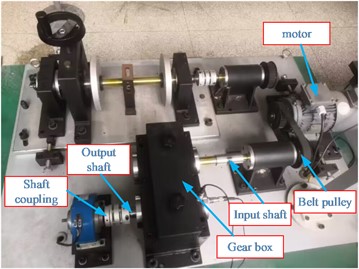
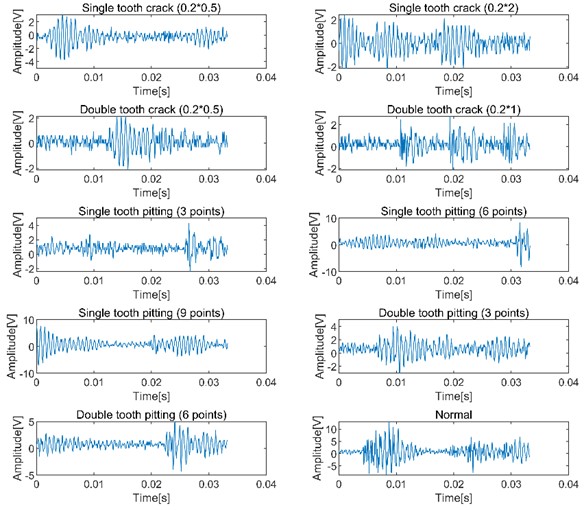
Among them, the number of teeth of the large gear of the gearbox is 75, the number of teeth of the small gear is 55, and the modulus is 2. In the experiment, the wire electric discharge cutting process was used to make faults on the large gear. By replacing the faulty gear in the gearbox, a total of 10 different gear states were simulated: normal state, crack fault and pitting fault, including faults at different points. For single-tooth and double-tooth faults, the faulty parts are shown in Fig. 14. Vibration data in different states is collected by the acceleration sensor installed on the gearbox. The motor speed is 1500 r/min, the sampling frequency is set to 12,800 Hz, and the sampling time is set to 10 s. A total of 128,000 data points are obtained for each state. In the experiment, 400 data points were selected as the data of a sample, and the number of fault samples of each type was 320 by using non-overlapping division. The samples were divided into training set, verification set and test set according to 7:1:2. Table 4 shows the experimental data sets have different numbers of fault points and different damage diameters (width or diameter×depth) to generate detailed information of different types of faults. Fig. 15 shows the original waveform diagram of the vibration signal measured under 10 types of gears.
Fig. 14Gear failure parts
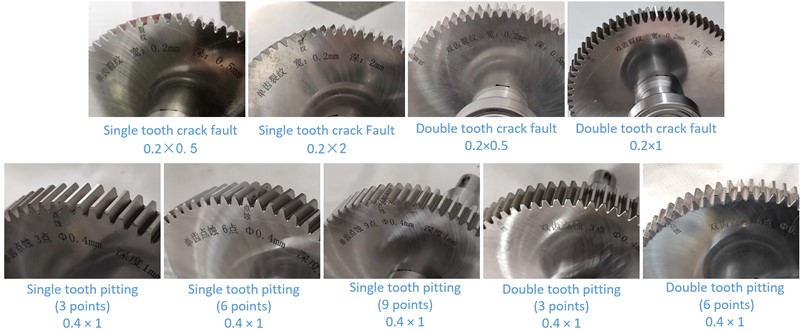
Fig. 15Original waveform diagram of gear vibration signal in different states
7.2. Analysis of experimental results
Fig. 16 shows the output results of the test set accuracy by using the proposed method same as section 6 and the proposed network model to conduct 10 experiments on the data respectively. The red line represents the accuracy using the proposed method and the blue line represents the accuracy using CNN directly. The average accuracy rate of the proposed method’ fault classification is 98.96 %, the highest accuracy rate is 99.69 %, and the lowest accuracy rate is 98.13 %. However, the average diagnostic accuracy of the CNN network was 95.41 %, and the highest accuracy was 97.19 %. It can be seen that this method can also achieve satisfactory classification results in the fault diagnosis of gears, and can effectively improve the diagnostic accuracy of the CNN network.
Table 4Gear failure dataset description
Fault type | Failure points | Damage diameter | sample length | Number of samples | Sample division | Label |
Normal | – | – | 400 | 320 | 224/32/64 | 0 |
Single tooth crack fault | – | 0.2×0.5 | 400 | 320 | 224/32/64 | 1 |
– | 0.2×2 | 400 | 320 | 224/32/64 | 2 | |
Double tooth crack fault | – | 0.2×0.5 | 400 | 320 | 224/32/64 | 3 |
– | 0.2×1 | 400 | 320 | 224/32/64 | 4 | |
Single tooth pitting fault | 3 Point | Ø0.4×1 | 400 | 320 | 224/32/64 | 5 |
6 Point | Ø0.4×1 | 400 | 320 | 224/32/64 | 6 | |
9 Point | Ø0.4×1 | 400 | 320 | 224/32/64 | 7 | |
Double tooth pitting fault | 3 Point | Ø0.4×1 | 400 | 320 | 224/32/64 | 8 |
6 Point | Ø0.4×1 | 400 | 320 | 224/32/64 | 9 |
Fig. 16Test set accuracy for ten trials
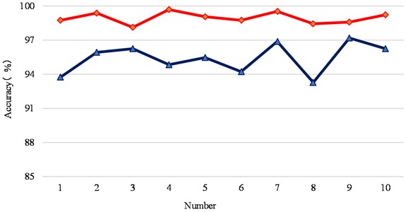
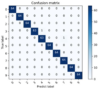
Fig. 17The proposed method is used to visualize the multi-class confusion matrix under the gear dataset
a) CNN network model multi-class confusion matrix visualization
b) Proposed model multi-class confusion matrix visualization
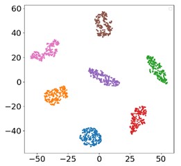
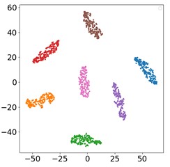
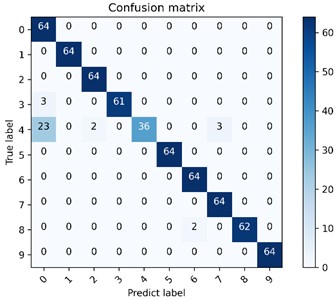
Fig. 17 and Fig. 18 are the multi-class confusion matrix and t-SNE feature visualization of the results obtained in the fourth of 10 experiments of this method, respectively. The recognition accuracy rate of the test set based on the proposed method is 99.69 %, and the error rate is 0.31 %. Among them, one real category 3 is misclassified to category 4 and one real category 4 is misclassified to category 7, and only one sample of each was misclassified. However, the accuracy of the CNN diagnostic model is only 94.84 %. It can also be seen from the t-SNE figure that the proposed method can cluster and identify better than the CNN network model, and its feature classes are more concentrated, which further proves that the proposed method can effectively improve the classification accuracy of CNN for gear fault diagnosis.
Fig. 18The proposed method is used for t-SNE feature visualization under the gear dataset
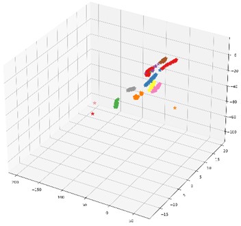
a) Feature visualization of the last fully connected layer of the CNN network model
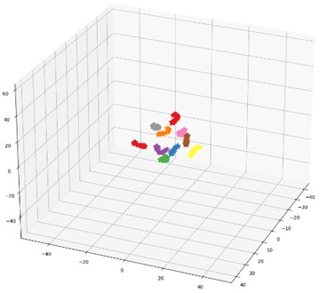
b) Feature visualization of the last fully connected layer of the proposed method’ network model
8. Conclusions
In order to solve the problem that CNN's excellent classification ability depends on a large number of data sample, a convolutional neural network intelligent diagnosis method based on SK-CAM is proposed. SK is used for preprocessing, and the obtained two-dimensional fast spectral kurtosis graph is converted into one-dimensional kurtosis time domain sample and used as the input of CNN, which reduces the difficulty of network feature learning. The introduction of CAM module increases the weight of network channel and adaptively eliminates the interference of invalid features. The accuracy of fault identification can reach 99.8 % by using 1HP data set from western reserve university. The smaller sample data sets are verified by experiment and the results show that this method still has high classification accuracy under smaller data sets. At the same time, the experiment under different load also achieved good diagnostic effect. Besides, the gear fault experiment data set is also used to further verify the excellent performance of the proposed method. Therefore, this method has higher precision and better generalization performance.
The paper mainly solves the fault diagnosis of rolling element bearing or gear under constant speed. In the future research, the order tracking analysis method being suitable for analyzing variable speed conditions will be combined with the proposed method to extend the research for fault diagnosis of rotating machinery working on variable speed condition, and make the proposed method more universal in engineering application.
References
-
R. Liu, B. Yang, E. Zio, and X. Chen, “Artificial intelligence for fault diagnosis of rotating machinery: A review,” Mechanical Systems and Signal Processing, Vol. 108, pp. 33–47, Aug. 2018, https://doi.org/10.1016/j.ymssp.2018.02.016
-
Y. Li, K. Ding, G. He, and X. Jiao, “Non-stationary vibration feature extraction method based on sparse decomposition and order tracking for gearbox fault diagnosis,” Measurement, Vol. 124, pp. 453–469, Aug. 2018, https://doi.org/10.1016/j.measurement.2018.04.063
-
Z. Liu, J. Wang, L. Duan, T. Shi, and Q. Fu, “Infrared image combined with CNN based fault diagnosis for rotating machinery,” in 2017 International Conference on Sensing, Diagnostics, Prognostics and Control (SDPC), pp. 137–142, Aug. 2017, https://doi.org/10.1109/sdpc.2017.35
-
S. Chen, Y. Meng, H. Tang, Y. Tian, N. He, and C. Shao, “Robust deep learning-based diagnosis of mixed faults in rotating machinery,” IEEE/ASME Transactions on Mechatronics, Vol. 25, No. 5, pp. 2167–2176, Oct. 2020, https://doi.org/10.1109/tmech.2020.3007441
-
Y. Cheng, M. Lin, J. Wu, H. Zhu, and X. Shao, “Intelligent fault diagnosis of rotating machinery based on continuous wavelet transform-local binary convolutional neural network,” Knowledge-Based Systems, Vol. 216, p. 106796, Mar. 2021, https://doi.org/10.1016/j.knosys.2021.106796
-
R. Liu, F. Wang, B. Yang, and S. J. Qin, “Multiscale kernel based residual convolutional neural network for motor fault diagnosis under nonstationary conditions,” IEEE Transactions on Industrial Informatics, Vol. 16, No. 6, pp. 3797–3806, Jun. 2020, https://doi.org/10.1109/tii.2019.2941868
-
R. Bai, Q. Xu, Z. Meng, L. Cao, K. Xing, and F. Fan, “Rolling bearing fault diagnosis based on multi-channel convolution neural network and multi-scale clipping fusion data augmentation,” Measurement, Vol. 184, p. 109885, Nov. 2021, https://doi.org/10.1016/j.measurement.2021.109885
-
Z. Wang, Y. Yin, and R. Yin, “Multi-tasking atrous convolutional neural network for machinery fault identification,” The International Journal of Advanced Manufacturing Technology, Vol. 124, No. 11-12, pp. 4183–4191, Jun. 2022, https://doi.org/10.1007/s00170-022-09367-x
-
H. Wang, C. Liu, W. Du, and S. Wang, “Intelligent diagnosis of rotating machinery based on optimized adaptive learning dictionary and 1DCNN,” Applied Sciences, Vol. 11, No. 23, p. 11325, Nov. 2021, https://doi.org/10.3390/app112311325
-
Y. Shao, X. Yuan, C. Zhang, Y. Song, and Q. Xu, “A novel fault diagnosis algorithm for rolling bearings based on one-dimensional convolutional neural network and INPSO-SVM,” Applied Sciences, Vol. 10, No. 12, p. 4303, Jun. 2020, https://doi.org/10.3390/app10124303
-
T. Jin, C. Yan, C. Chen, Z. Yang, H. Tian, and S. Wang, “Light neural network with fewer parameters based on CNN for fault diagnosis of rotating machinery,” Measurement, Vol. 181, p. 109639, Aug. 2021, https://doi.org/10.1016/j.measurement.2021.109639
-
M. Demetgul, K. Yildiz, S. Taskin, I. N. Tansel, and O. Yazicioglu, “Fault diagnosis on material handling system using feature selection and data mining techniques,” Measurement, Vol. 55, pp. 15–24, Sep. 2014, https://doi.org/10.1016/j.measurement.2014.04.037
-
G. M. Nita, “Spectral Kurtosis statistics of transient signals,” Monthly Notices of the Royal Astronomical Society, Vol. 458, No. 3, pp. 2530–2540, May 2016, https://doi.org/10.1093/mnras/stw550
-
R. Dwyer, “Detection of non-Gaussian signals by frequency domain kurtosis estimation,” in IEEE International Conference on Acoustics, Speech, and Signal Processing, p. 1983, Jan. 2024, https://doi.org/10.1109/icassp.1983.1172264
-
S. Wan, X. Zhang, and L. Dou, “Compound fault diagnosis of bearings using an improved spectral kurtosis by MCDK,” Mathematical Problems in Engineering, Vol. 2018, pp. 1–12, Jan. 2018, https://doi.org/10.1155/2018/6513045
-
S. Jing, J. Yuan, X. Li, and J. Leng, “Weak fault feature identification for rolling bearing based on EMD and spectral kurtosis method,” in 2018 International Conference on Information Systems and Computer Aided Education (ICISCAE), pp. 235–239, Jul. 2018, https://doi.org/10.1109/iciscae.2018.8666841
-
J. Antoni, “Fast computation of the kurtogram for the detection of transient faults,” Mechanical Systems and Signal Processing, Vol. 21, No. 1, pp. 108–124, Jan. 2007, https://doi.org/10.1016/j.ymssp.2005.12.002
-
Y.-J. Huang, A.-H. Liao, D.-Y. Hu, W. Shi, and S.-B. Zheng, “Multi-scale convolutional network with channel attention mechanism for rolling bearing fault diagnosis,” Measurement, Vol. 203, p. 111935, Nov. 2022, https://doi.org/10.1016/j.measurement.2022.111935
-
H. Wang, Z. Liu, D. Peng, and Y. Qin, “Understanding and learning discriminant features based on multiattention 1DCNN for wheelset bearing fault diagnosis,” IEEE Transactions on Industrial Informatics, Vol. 16, No. 9, pp. 5735–5745, Sep. 2020, https://doi.org/10.1109/tii.2019.2955540
-
M. Beibei, S. Yanxia, W. Dinghui, and Z. Zhipu, “Three level inverter fault diagnosis using EMD and support vector machine approach,” in 12th IEEE Conference on Industrial Electronics and Applications (ICIEA), pp. 1595–1598, Jun. 2017, https://doi.org/10.1109/iciea.2017.8283093
-
S. Huang, J. Tang, J. Dai, and Y. Wang, “Signal status recognition based on 1DCNN and its feature extraction mechanism analysis,” Sensors, Vol. 19, No. 9, p. 2018, Apr. 2019, https://doi.org/10.3390/s19092018
-
L. Wan, Y. Chen, H. Li, and C. Li, “Rolling-element bearing fault diagnosis using improved LeNet-5 network,” Sensors, Vol. 20, No. 6, p. 1693, Mar. 2020, https://doi.org/10.3390/s20061693
-
F. Wei, G. Wang, B. Ren, J. Ge, and Y. Wang, “Multisensor fused fault diagnosis for rotation machinery based on supervised second-order tensor locality preserving projection and weighted k-nearest neighbor classifier under assembled matrix distance metric,” Shock and Vibration, Vol. 2016, pp. 1–14, Jan. 2016, https://doi.org/10.1155/2016/1212457
Cited by
About this article

The authors have not disclosed any funding.
The datasets generated during and/or analyzed during the current study are available from the corresponding author on reasonable request.
Liang Chen: writing. Simin Li: algorithm implementation and programming. Peijun Li: conception and architecture. Yutao Liu: signal processing. Renqi Chang: literature research.
The authors declare that they have no conflict of interest.
