Abstract
Although, deep learning has been successfully used for fault diagnosis of rolling bearing by training large-scale data, the acquisition of large-scale fault data requires a high cost. For small-scale data, the precision of network model will decrease with the deepening of network layers. Aiming at above issue, a convolutional neural network algorithm based on transfer learning model is proposed. First, the overlap sampling of rolling bearing fault signals are used to enhance the datasets, and the transfer learning model is pre-trained on standard-scale dataset to obtain the initial network parameters, that will be used to extract bearing fault features from small-scale dataset. The effects of data scale and fault categories on model accuracy are discussed based on the comparison and verification on public bearing fault dataset. The results show that the proposed method in this paper can achieve high-precision with a small computational cost on fault identification of small-scale fault data, and the method shows popularization value for the analysis of small-scale datasets in other areas.
1. Introduction
Affected by harsh working conditions, the key components of rotating machinery, such as bearings and gears, are more prone to failure, which will caused a fatal impact on the safe operation of the whole machinery system [1]. It is of great significance to identify the fault mode in time for the safe and reliable operation of the system.
With the development of machine learning technology, intelligent fault diagnosis methods can directly provide more reliable diagnosis results by training original vibration signals, which can greatly improve the accuracy and efficiency of fault identification. The improvement of computing power makes large-scale-based data-driven intelligent fault diagnosis methods gradually become a research issue, such as deep learning technology. Shao [2] applied deep convolutional neural network (DCNN) to image representation, and proposed a multi-signal model based on deep learning, which overcome over-fitting problem to a certain extent. Qiu [3] applied DCNNs and support vector machines (SVM) to diagnose faults in gearboxes, respectively, and the results showed that DCNNs were more suitable for solving the problem of multi-fault state recognition.
In addition, other intelligent recognition algorithms are also studied and applied to the field of fault diagnosis. For example, linear discriminant analysis (LDA) [4], deep belief network (DBN) [5], recurrent neural network (RNN) [6-8] and so on. Although deep learning network has a high recognition effect on large-scale fault data, the acquisition cost of labeled fault data in engineering is quite high. How to improve the bearing fault identification accuracy and stability when the data scale changes has gradually become a challenge in the field of mechanical fault diagnosis. Due to the over-fitting problem, when the size of the data set is reduced, the accuracy and robustness of the general convolutional neural network (CNN) will decrease [9]. The training time of deep CNN will be long as the layers depth. In order to further improve the recognition accuracy and efficiency of CNN for small-scale fault data sets in the mechanical field, mechanical fault diagnosis methods based on transfer learning have gradually become a research hotspot.
For our present purpose, transfer learning has been successfully applied in image recognition, speech recognition, text recognition and other fields [10], and it is worthy of further exploration in the field of intelligent fault diagnosis in rolling bearings. Xu [11] converted time-domain signals into images, and proposed an online fault diagnosis method based on LeNet-5 for deep migration learning, which achieved the desired accuracy in a limited time. Long Wen [12] proposed a new deep transfer learning method based on sparse autoencoders, and the fault prediction accuracy on the motor bearing data set is better than the traditional method. An Z [13] proposed a three-layer network model based on RNN and transfer learning, which realized the fault diagnosis of the variable sequence of motor system faults under different working conditions. At present, most research on transfer learning combines traditional feature extraction with transfer learning. These studies are mainly for large-scale data sets. The classification of small-scale fault data still has the problems of low accuracy, complex modeling, slow diagnosis, and low efficiency, which need to be studied [14].
In connection with the problem of the small scale of rolling bearing fault data, the paper proposes a fault identification method based on transfer learning. First, the overlap sampling of rolling bearing fault signals are used to enhance the datasets, and the Gaussian noise are used to expand the training samples to increase the noise immunity of the network. The transfer learning model is pre-trained on standard-scale dataset to obtain the initial network parameters, that will be used to extract bearing fault features from small-scale dataset. In addition, the classification layer is reconstructed and the parameters are fine-tuned during the training process to meet the new classification requirements. Finally, we compare the network performance of the proposed method with traditional methods.
2. Deep transfer learning model
2.1. Transfer learning model
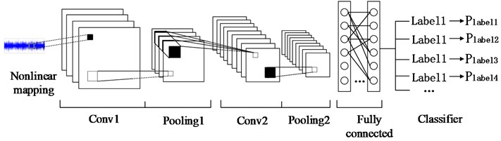
Fig. 1 shows the typical structure of CNN, which is usually composed of convolutional layer, pooling layer and fully connected layer. Many classic deep learning networks are inspired by this structure to train large-scale data sets by deepening the network. Due to the problem of overfitting, the fault recognition effect of general deep convolutional neural networks becomes worse when training on a small-scale dataset.
Fig. 1Typical structure of CNN
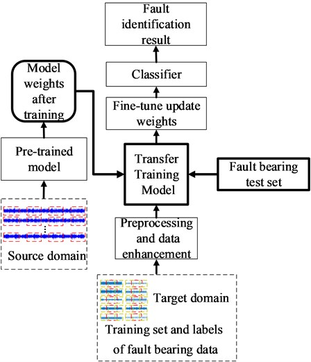
Generally, a new neural network model can be trained by transferring the trained model parameters to the new model. Considering that most data or tasks are related, the knowledge learned by the model can be shared with the new model in a certain way through transfer learning to speed up and optimize the learning efficiency of the model. The flow chart of the proposed mothed is shown in Fig. 2.
The whole process is divided into two parts. In the pre-training process, the original time-domain image of vibration signal is read by classification, and the category quantity is obtained and the known label is given by one-hot coding. Then the data set is randomly arranged and divided into training set and test set at a ratio of 7:3. Secondly, the training set image is input into the pre-training model to verify the recognition rate on the test set after a certain number of iterations. Finally, the network parameters will be saved. In the network transfer part, the network parameters of each pre-training layer are read to recover network, and then a new network structure will be formed through adding a fully connected layer. Secondly, the small-scale dataset in the target domain is divided into training dataset and testing dataset. Then the training dataset is standardized and overlapped to be saved as the time domain image. Finally, the bearing vibration signal that in the target domain is identified.
Fig. 2Fault identification flow chart of transfer learning
The overall structure of transfer learning network of rolling bearing fault identification is shown in Fig. 3. The network consists of two main parts. The first part is the preparation stage of the migration model parameters. The migration model is trained on the large-scale standard dataset, and the trained model parameters are saved. In this network, the larger two dimensional convolution is divided into several smaller one dimensional convolution, which can reduce the over-fitting and increases the nonlinear expression ability of the model with asymmetric convolution structure. The second part is the training and testing stage of fault diagnosis network, the small-scale original time domain fault signal will be overlap sampled, and they will be input to the migration model through a layer of digital filter denoising. The migration model is initialized by calling the weights prepared by the first step of the pre-training, and all the previously trained convolution layer will be frozen. The last four layers will be retrained and adjusted for the training dataset of the rolling bearing. In order to reduce over-fitting, dropout [15] is added to the fully connected layer. Softmax classifier is used to get the result in the end.
2.2. Related theories
Softmax classifier with a polynomial distribution model is used in the algorithm proposed in this paper, which can distinguish multiple mutually exclusive categories. Since the fault diagnosis corresponding to the experimental data is single label and multiple classification, the cross-entropy is used as the loss function to calculate the loss of a training sample batch, which can be expressed as following:
where is the number of categories. is the number of samples in the current training batch. is the actual label of the samples, and is the label predicted by the model.
Fig. 3The proposed transfer learning model structure
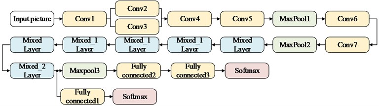
a) Transfer network structure
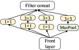
b) Mixed layer
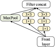
c) Mixed_1 layer
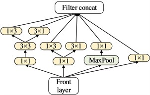
d) Mixed_2 layer
When the CNN is continuously deepened and widened, a lot of time and computer resources will be required for network training. Although distributed parallel training can be used to accelerate the learning of the model, the required computing resources have not been reduced. The method based on transfer learning proposed in this paper not only reduces the calculation time and network complexity by calling network parameters that have good effects on large-scale data sets, but also selects Adam optimization algorithms that require less resources and faster convergence to accelerate model learning. When looking for the minimum value of a complex function, the direct derivative is too complicated and can usually be calculated by iteration. The Adam algorithm is used to perform gradient descent on the objective function, and the optimized objective function can be given as:
where is the number of training batches, is the true value, and is the prediction model. The first item is the empirical risk, which is the average loss of on the training dataset. It can reflect the degree of fit of the model to the historical data. The second item is the structural risk, which measures the complexity of the model. The coefficient is used to adjust its importance. Assuming is the objective function, the gradient update formula can be expressed as:
where is the parameter value at the time when the solution is required. is the learning rate, and the initial value is 0.001, which can be used to control the step sizes. is the first-order moment estimation of the gradient of the function, and is the second-order moment estimation corresponding correction value.
3. Establishment of rolling bearing fault data set
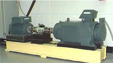
In this paper, the experimental datasets come from the Case Western Reserve University (CWRU) Bearing Data Center (http://csegroups.case.edu/bearingdatacenter). The rolling bearing dataset has successfully provided proof for many mainstream fault diagnosis algorithms of rolling bearing in the current research literature [16-18]. Fig. 4 is the test principle diagram of the vibration signal of the CWRU rolling bearing dataset. The testing device is mainly composed of induction motor, torque sensor, power meter, accelerometer and control system. The testing bearing is a deep groove ball bearing (6205-2RS JEM SKF), which is installed at the drive end of the induction motor.
Fig. 4Principle of vibration signal testing of bearing
The drive end dataset is selected in this research. Three different fault types are rolling element fault (BA), inner ring fault (IR) and outer ring fault (OR), and each fault type contains three different fault sizes, 0.007 inch, 0.014 inch, and 0.021 inch, which can represents different fault levels of the damage. Different time-domain vibration signals were recorded under three different motor loads of 1 hp, 2 hp and 3 hp. As shown in Table 1, the dataset is divided into training dataset and testing dataset in the network. There are totally 10 fault types for each working condition including the healthy state of bearing and 9 different fault signals, which are labeled with ten number from 0 to 9. Under each fault condition, the original vibration signal of the first 10 seconds is truncated into 540 data pieces, and the length of each data piece is 600 at most. In each dataset, there are totally 5400 data pieces for these 10 fault types.
Table 1Rolling bearing failure data set
Fault location | – | BA | IR | OR | Load | |||||||
Label | 0 | 1 | 2 | 3 | 4 | 5 | 6 | 7 | 8 | 9 | /hp | |
Diameter (inch) | 0.007 | 0.014 | 0.021 | 0.007 | 0.014 | 0.021 | 0.007 | 0.014 | 0.021 | |||
A | Train | 540 | 540 | 540 | 540 | 540 | 540 | 540 | 540 | 540 | 540 | 1 |
Test | 108 | 108 | 108 | 108 | 108 | 108 | 108 | 108 | 108 | 108 | ||
B | Train | 540 | 540 | 540 | 540 | 540 | 540 | 540 | 540 | 540 | 540 | 2 |
Test | 108 | 108 | 108 | 108 | 108 | 108 | 108 | 108 | 108 | 108 | ||
C | Train | 540 | 540 | 540 | 540 | 540 | 540 | 540 | 540 | 540 | 540 | 3 |
Test | 108 | 108 | 108 | 108 | 108 | 108 | 108 | 108 | 108 | 108 | ||
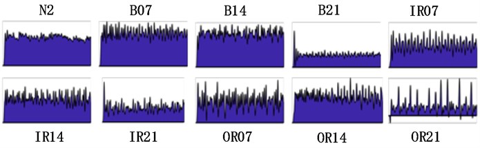
The training data of the original time-domain vibration signal with a length of 600 under different fault conditions is shown in Fig. 5(a). It can be seen that it is difficult to identify different bearing faults subjectively from the original vibration signal, especially when the fault occurs on the rolling element. The feature maps after the fast Fourier transform corresponding to the training data are shown in Fig. 5(b). Although the peak values are different, the signals are also very messy. The time-frequency diagrams obtained from the corresponding training data slice are shown in Fig. 5(c). The data are converted into time-domain images with richer information, and the two-dimensional convolution operation is more convenient to extract useful fault features.
Fig. 5Different signal forms under different fault scales
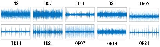
a) Original vibration signal
b) FFT Feature map
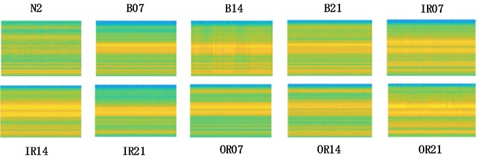
c) Time-frequency diagram
4. Faults recognition results and analysis
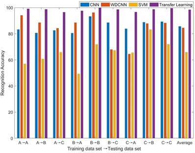
In order to verify the performance of the proposed network under different motor load conditions, the original vibration data collected under 1 hp, 2 hp and 3 hp motor loads are defined as data sets A, B, and C, as shown in Table 1. At the same time, the proposed network is trained on 70 % of data set, and the other 30 % test sets from three different data sets are used to test the trained network. As shown in Table 2, we use 9 different dataset representations to represent these combined operations. For example, B→C means that the network is trained on dataset B, and 30 % data are taken randomly from the dataset C for testing.
4.1. Accuracy evaluation
In order to test the performance of the proposed method, the recognition accuracy of the traditional methods, such as CNN, WDCNN, SVM algorithm, are compared with the proposed method. The recognition accuracy is defined as the ratio of the number of correctly identified fault data to the total number of test data. In order to reduce the impact of training randomness, each method is tested three times, and the average recognition accuracy is taken as the algorithm accuracy result. the average recognition accuracy trend of algorithm representation is shown in Fig. 6. It can be seen that when the training dataset and the testing dataset come from the same load, the four networks all show better performance. The average recognition accuracy of general CNN is much higher than that of WDCNN and support vector machine, especially when the training dataset and testing dataset are different, the average recognition accuracy of WDCNN and support vector machine is greatly reduced. The rolling bearing fault diagnosis method based on the migration model proposed in this paper has the best comprehensive performance. No matter when training dataset and the testing dataset from the same load condition, or when the two are from different loads, the average recognition accuracy of this algorithm is higher than the other three traditional methods, which can reach 98.5 %.
Table 2Representation of different fault datasets
Train set | Test set | Combination |
A (1 hp) | A | A→A |
B | A→B | |
C | A→C | |
B (2 hp) | A | B→A |
B | B→B | |
C | B→C | |
C (3 hp) | A | C→A |
B | C→B | |
C | C→C |
Table 3Accuracy comparison experiment
Data set train → test | CNN | WDCNN | SVM | Transfer learning |
Accuracy (%) | ||||
A→A | 83.33 | 94.20 | 57.15 | 99.25 |
A→B | 80.67 | 88.67 | 60.87 | 98.78 |
A→C | 82.71 | 84.33 | 65.95 | 96.55 |
B→A | 80.63 | 88.65 | 49.38 | 97.64 |
B→B | 93.33 | 96.33 | 72.00 | 99.89 |
B→C | 88.67 | 68.08 | 67.39 | 98.61 |
C→A | 83.87 | 64.67 | 65.67 | 96.67 |
C→B | 88.95 | 87.95 | 83.33 | 98.85 |
C→C | 89.40 | 88.40 | 72.11 | 99.68 |
Average | 85.73 | 84.59 | 65.98 | 98.50 |
Fig. 6Recognition accuracy trend
4.2. The influence of fault dataset scale
In order to verify the ability of the transfer learning-based network proposed in this paper to identify small-scale datasets, we take dataset A→B as an example to reduce the dataset size for getting small-scale datasets. The dataset size is reduced to 70 %, 40 %, 20 %, 10 % and 4 % of the total original dataset. It is worth noting that the same number of samples for each category is removed to form new dataset. Fig. 7 are the box diagrams of the experiment under five different datasets. In order to reduce the experimental error, ten experiments are carried out on each dataset. It can be seen intuitively that as the amount of dataset decreases, the overall recognition accuracy of the proposed method is not only higher than other methods, but also the recognition rate is stable. Since the error fluctuation range is smaller, the possibility of outliers of the results is also less.
Fig. 7Identification accuracy under different dataset size
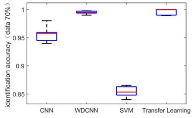
a) 70 %
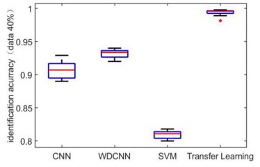
b) 40 %
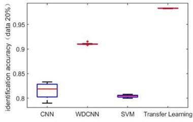
c) 20 %
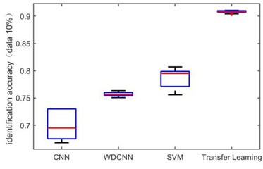
d) 10 %
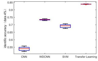
e) 4 %
4.3. The influence of the number of fault data categories
As to rolling bearing fault data, the accuracy of fault recognition based on transfer learning is affected to a certain extent by the data distribution and the amount of recognition categories. Generally, the more categories need to be classified, the more difficult it is to identify different faults as the fault dataset size decreases. Fig. 8 shows the error bar graph of the fault recognition accuracy on 10 groups of experiments. Where 3-3 indicates that there are three kinds of faults to be identified in source domain and target domain. It can be seen that when the number of fault kinds in source domain is equal to that in target domain, the transfer method proposed in this paper can achieve an average recognition rate of 98 %. As the categories increase, the algorithm maintains a certain degree of stability.
Fig. 8Multi-class fault recognition error bar graph
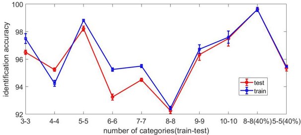
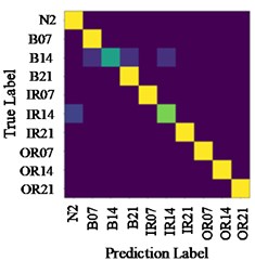
Fig. 9Confusion matrix of test results on data set with load 2
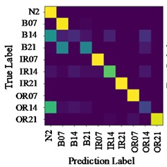
a) CNN (A→B)
b) Proposed method (C→A)
c) Proposed method (A→B)
Fig. 9 shows the identification results confusion matrix of two methods. Confusion matrix is a kind of specific matrix, which is used to present the visual effect of algorithm performance. Each row represents the actual category, and each column represents the prediction category. The color scale bar on the right side ranges from 0 to 1, indicating the proportion that classified as in the total number of samples. When all are classified as by the model, the corresponding color we can see is yellow. For that reason, all correct predictions are on the diagonal, which is called the recall rate (or sensitivity) of the model:
where represents the number of correctly identified samples of a certain category, and represents the number of incorrectly identified samples of this category.
From Fig. 9(a), it can be seen that some bearing rolling element faults with 0.14-inch diameter are mistakenly identified as 0.007-inch rolling element faults, and some are identified as 0.021-inch rolling element faults. This is because that these types of fault features are similar, and common CNN network cannot identify accurately. However, when the proposed method is used, most of them can be accurately classified. As shown in Fig. 9(c), on the data set A→B, the confusion matrix values of the experimental results are concentrated in the diagonal region, and the recall rate is 1.0. Therefore, it is feasible to transfer existing high-performance network weight adjustments to help new task to complete fault identification goal, and the result is more accurate than that of shallow CNN.
5. Conclusions
Aiming at the problem of low fault recognition accuracy and low modeling efficiency caused by small amount of bearing fault dataset, a DCNN algorithm based on migration model is formulated in this paper. Firstly, the fault datasets are enhanced to reduce the dependence of the model on the amount of data. The transfer network parameters are pre-trained on standard datasets, and the classification layer is redesigned. Finally, the method is verified on the public bearing fault dataset, and comparative analysis is carried out in a variety of situations to study the influence of the fault dataset sizes and the amount of fault categories on the recognition accuracy. The results show that the proposed methods can not only realize high-precision fault identification of small-scale fault datasets of rolling bearing, but also show better stability than traditional methods when the fault dataset sizes change.
References
-
Huang X., Wen G., Liang L., Zhang Z., Tan Y. Frequency phase space empirical wavelet transform for rolling bearings fault diagnosis. IEEE Access, Vol. 7, 2019, p. 86306-86318.
-
Shao S., Yan R., Lu Y., Wang P., Gao R. X. DCNN-based multi-signal induction motor fault diagnosis. IEEE Transactions on Instrumentation and Measurement, Vol. 69, Issue 6, 2020, p. 2658-2669.
-
Qiu G., Gu Y., Cai Q. A deep convolutional neural networks model for intelligent fault diagnosis of a gearbox under different operational conditions. Measurement, Vol. 145, 2019, p. 94-107.
-
Li M., Yuan B. 2D-LDA: A statistical linear discriminant analysis for image matrix. Pattern Recognition Letters, Vol. 26, Issue 5, 2005, p. 527-532.
-
Li W., Shan W., Zeng X. Bearing fault classification and recognition based on deep belief network. Journal of Vibration Engineering, Vol. 29, Issue 2, 2016, p. 340-347.
-
Zhao R., Yan R., Chen Z., Mao K., Wang P., Gao R. Deep learning and its applications to machine health monitoring. Mechanical Systems and Signal Processing, Vol. 115, 2016, p. 213-237.
-
Liu H., Zhou J., Zheng Y., Jiang W., Zhang Y. Fault diagnosis of rolling bearings with recurrent neural network-based autoencoders. ISA Transactions, Vol. 77, 2018, p. 167-178.
-
Deng W., Yao R., Zhao H., Yang X., Li G. A novel intelligent diagnosis method using optimal LS-SVM with improved PSO algorithm. Soft Computing, Vol. 23, Issue 7, 2017, p. 2445-2462.
-
Cao P., Zhang S., Tang J. Pre-processing-free gear fault diagnosis using small datasets with deep convolutional neural network-based transfer learning. IEEE Access, Vol. 6, 2017, p. 26241-26253.
-
Chen Y. Multiple-level biomedical event trigger recognition with transfer learning. BMC Bioinformatics, Vol. 20, Issue 1, 2019, p. 459.
-
Xu G., Liu M., Jiang Z., Shen W., Huang C. Online fault diagnosis method based on transfer convolutional neural networks. IEEE Transactions on Instrumentation and Measurement, Vol. 69, Issue 2, 2020, p. 509-520.
-
Wen L., Gao L., Li X. A new deep transfer learning based on sparse auto-encoder for fault diagnosis. IEEE Transactions on Systems, Man, and Cybernetics: Systems, Vol. 49, Issue 1, 2019, p. 136-144.
-
An Z., Li S., Xin Y., Xu K., Ma H. An intelligent fault diagnosis framework dealing with arbitrary length inputs under different working conditions. Measurement and Technology, Vol. 30, Issue 12, 2019, p. 125107.
-
Dogo E. M., Afolabi O. J., Nwulu N. I. A comparative analysis of gradient descent-based optimization algorithms on convolutional neural networks. International Conference on Computational Techniques, Electronics and Mechanical Systems (CTEMS), 2018.
-
Fan G., Li J., Hao H. Vibration signal denoising for structural health monitoring by residual convolutional neural networks. Measurement, Vol. 157, 2020, p. 107651.
-
Ma P., Zhang H., Fan W., Wang C. A diagnosis framework based on domain adaptation for bearing fault diagnosis across diverse domains. ISA Transactions, Vol. 99, 2020, p. 465-478.
-
Lou X., Loparo K. A. Bearing fault diagnosis based on wavelet transform and fuzzy inference. Mechanical Systems and Signal Processing, Vol. 18, Issue 5, 2004, p. 1077-1095.
-
Li X., Ma J., Wang X., Wu J., Li Z. An improved local mean decomposition method based on improved composite interpolation envelope and its application in bearing fault feature extraction. ISA Trans, Vol. 97, 2020, p. 365-383.
About this article

The authors acknowledge the supports by the National Natural Science Foundation of China under Grant 51705494 and the Natural Science Foundation of Zhejiang Province, China, under Grant LQ17E050005, and by the Key research and development program of Zhejiang Province, China, under Grant 2020C01054.
