Abstract
Rolling element bearings (REBs) are vital parts of rotating machinery across various industries. For preventing breakdowns and damages during operation, it is crucial to establish appropriate techniques for condition monitoring and fault diagnostics of these bearings. The development of machine learning (ML) brings a new way of diagnosing the fault of rolling element bearings. In the current work, ML models, namely, Support Vector Machine (SVM) and K-Nearest Neighbor (KNN), are used to classify the faults associated with different ball bearing elements. Using open-source Case Western Reserve University (CWRU) bearing data, machine learning classifiers are trained with extracted time-domain and frequency-domain features. The results show that frequency-domain features are more convincing for the training of ML models, and the KNN classifier has a high level of accuracy compared to SVM.
1. Introduction
Fault detection and diagnosis of rotating machinery play an essential role in maintenance planning, human safety, and cost reduction in modern industrial systems. As the rolling element bearings are an integral component of rotating machinery, their failure is a leading cause of machinery malfunction [1]. Bearing failures account for 30 to 40 percent of total machinery failure. These defects, if detected early enough, can help prevent accidents [2]. Various methods for diagnosing bearing faults have been employed, such as acoustic emission [3], vibration [4], motor current [5], thermography [6] and, so on. The microphone sensor of a mobile phone is used to record acoustic data and investigate bearing health issues [3]. However, the approach is limited by the weak frequency response of the integrated microphone in low-frequency bands, which is especially problematic for low voltage motors. An adaptive noise canceling method is proposed for diagnosing bearing faults in induction motors [7]. Vibration-based diagnostics is the most extensively utilized technique for early failure identification in induction motors among several diagnostic methods [8-9]. An artificial neural network (ANN) was used to estimate the bearing condition [8]. It has been discovered that successful bearing diagnosis can be achieved by applying suitable measurement and processing of motor vibration signals. Bearing defect detection based on Hidden Markov Modeling (HMM) using vibration signal is proposed in reference [10]. An amplitude demodulated signal is used for feature extraction and training HMMs to estimate normal and faulty bearings. Envelope analysis, often known as High-Frequency Resonance Technique (HFRT), is the most widely used frequency-domain approach for bearing defect diagnostics [11]. Due to mechanical components, however, the technology suffers from a low signal-to-noise ratio and the existence of a high number of frequencies. Furthermore, the procedure necessitates the determination of bearing defect frequencies in advance.
Many research findings support the machine learning approach in machinery fault diagnosis as the ML methods are more competitive than signal-based methods [12-15]. Machine learning characteristics collected from data are more objective than signal-based methods. Furthermore, the accuracy criterion of fault diagnosis is more helpful in selecting fault diagnosis methods. In the current work, vibration signals from a bearing are gathered under both healthy and faulty conditions. Various time and frequency-domain features are extracted from the data and are used to distinguish different bearing conditions using the SVM and KNN classifiers.
1.1. Support Vector Machine (SVM)
Support Vector Machines (SVMs), also known as support vector networks [12], are supervised learning models that examine data for classification and regression analysis in machine learning. SVM, which is based on statistical learning frameworks, is one of the most reliable prediction approaches. An SVM training algorithm creates a model that assigns new examples to one of two categories, making it a non-probabilistic binary linear classifier, given a series of training examples, each marked as belonging to one of two categories.
Let some data points are assigned to one of two classes, and the purpose is to determine that a new data point will be allocated to which class. A data point is viewed as a -dimensional vector (a list of numbers) in support-vector machines, and one wants to know if such points can be separated with a -dimensional hyperplane. This is termed a linear classifier. Numerous hyperplanes may be used to categorize the data. If such a hyperplane exists, it is called a maximum-margin hyperplane. The linear classifier it thus defines is called a maximum-margin classifier. The hyperplane that represents the greatest separation, or margin, between the two classes is a viable choice as the best hyperplane. As shown in Fig. 1, the classes are not separated by the hyperplane 𝐻1. The hyperplane 𝐻2 has a slight advantage, but only by a short margin. With maximum success, the hyperplane 𝐻3 separates them by the widest possible margin.
1.2. K-Nearest Neighbor (KNN) algorithm
The K-Nearest Neighbor (KNN) algorithm is one of the most basic machine-learning algorithms [13]. It is a method of calculating the distance between two points [14]. Due to its simplicity and ease of implementation, this is a widely used classifier. It is a non-parametric classification and regression method. As seen in Fig. 2, this algorithm assumes that related entities are close to one another.
Fig. 1Different hyperplanes separating the two classes of data points
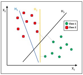
Fig. 2A demonstration of KNN algorithm
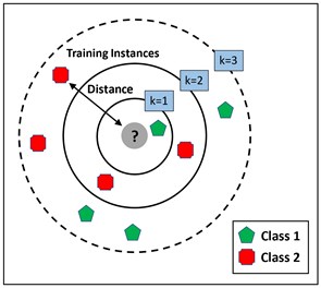
KNN determines the distance between two points using multiple techniques, such as Euclidian and Manhattan [15], based on the idea of similarity based on proximity or distance. However, Euclidian is the most generally used among all of these ways, and it can be represented by Eq. (1):
where , are two points in an dimensional Euclidian space.
KNN must be run several times with different values of to determine the chosen number of (the number of neighbors) for a given dataset. The value of should be selected to decrease the number of errors when making predictions from each run.
2. Bearing data description
Fig. 3 shows the CWRU test platform, including a 2-horsepower motor, dynamometer, torque sensor, and electronic control unit [16]. Experiments are performed with bearings having EDM-created single point defects with diameters of 7 mils, 14 mils, 21 mils, 28 mils, and 40 mils (1 mil = 0.001 inches). SKF bearings are used for the 7, 14, and 21 mils diameter faults, whereas NTN bearings are used for the 28 mils and 40 mils diameter faults.
Vibration data was acquired using accelerometers installed at the 12 o'clock position of the motor casing and processed in MATLAB (.mat) format. Signals were captured at a sampling frequency of 12 kHz for drive and fan end bearings and 48 kHz for drive end bearing faults.
Fig. 3Test stand of CWRU bearing data center [16]
![Test stand of CWRU bearing data center [16]](https://static-01.extrica.com/articles/22307/22307-img3.jpg)
2.1. Fault dataset
The ensembled dataset considered in this work for the performance analysis of ML models in classifying bearing faults comprises four categories of the bearing data: healthy bearing, inner race defect, outer race defect lying orthogonal to the load zone, and outer race defect located in the load zone. Twenty data samples, each of 3600 data points, are taken from all of the four categories, thus making 80 entries in the ensembled dataset. The detailed description of the ensembled dataset concerning the location of bearing, shaft speed, and assigned fault codes is given in Table 1.
Table 1Details of bearing dataset considered for fault classification
Bearing location | Motor load/shaft speed | Defect size | Bearing condition | Fault data designation | Fault code |
Drive end | 2 HP/ 1750 rpm | 21 mils (0.021″) | Healthy | Normal_2 | 1 |
Defective inner race | IR021_2 | 2 | |||
Defective outer race (Defect lying orthogonal to the load zone) | OR021@3_2 | 3 | |||
Defective outer race (Defect located in the load zone) | OR021@6_2 | 4 |
2.2. Fault features
A total of 18 time-domain and frequency-domain fault features extracted are used in different combinations to assess the accuracy of SVM and KNN models in classifying the bearing fault categories. The time-domain features used are clearance factor, crest factor, impulse factor, kurtosis, mean, peak value, RMS, SINAD, SNR, shape factor, skewness, standard deviation, approximate entropy, correlation dimension, and Lyapunov exponent. The features of the frequency-domain taken are peak amplitude, peak frequency, and band power.
3. Procedure
The step-wise methodology employed in the present work is presented in this section. First of all, the bearing data corresponding to fault categories of interest is ensembled. Numerous time-domain and frequency-domain features are then extracted from this ensembled data and also ranked. Finally, these features are selected in different combinations to train ML models to obtain their fault classification accuracy. The methodology’s workflow is depicted in Fig. 4.
Fig. 4The methodology used for bearing fault classification

3.1. Feature extraction
The time and frequency-domain features are extracted from the ensembled bearing data in MATLAB environment and are ranked in order of their relative significance to be used to train the ML classifiers. These features may all be used together or selectively in varying combinations to train ML models for the comparison of their accuracy in classifying the bearing faults. The accuracy results corresponding to each set of selected features are compared to identify the promising features and the classifier providing maximum accuracy.
3.2. Training of ML models
In the current study, the ML models are trained using the 𝑘-fold cross-validation approach. This method divides a dataset into k folds of equal size at random. The model is then fitted on the remaining 𝑘-1 folds after selecting one of the folds as the holdout set. The model is put to the test for the observations that were held out in the fold. The method is repeated k times, with a different set as the holdout set each time. 5-fold cross-validation is employed in the present analysis, thus splitting ensembled data of 80 entries into 5 equal-sized folds, each having random 16 sub datasets.
4. Results and discussion
After the features are extracted and the models are trained, the accuracy results of fault classification are obtained and presented in terms of scatter plot and confusion matrix with the selection of different features. The predictors that may distinguish the classes can be determined by plotting several predictors on the scatter plot. A scatter plot depicts the data before training the classifier, and the model prediction results are displayed once the classifier has been trained. RMS and skewness are considered as predictors in the present case. A confusion matrix can be used to detect the areas where the classifier has failed. The True Positive Rate (TPR) is defined as the percentage of correctly classified observations per true class. The False Negative Rate (FNR) is the proportion of observations that are wrongly categorized per true class. In the last two columns on the right, the plot gives summaries for each true class.
To train ML models, features both from the time-domain and frequency-domain are selected in the first trial. A combination of three non-linear time-domain features, namely, approximate entropy, correlation dimension, and Lyapunov exponent, are considered in the second feature set. In the last group, three frequency-domain features are used for model training. Figs. 5-7 show the scatter plots and confusion matrices for a few results of fault classification of SVM and KNN classifiers with three different feature sets. The corresponding accuracies obtained are reported in Table 2.
Fig. 5Scatter plot and confusion matrix for SVM classifier with the feature set 1
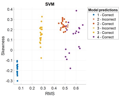

Fig. 6Scatter plot and confusion matrix for KNN classifier with the feature set 2
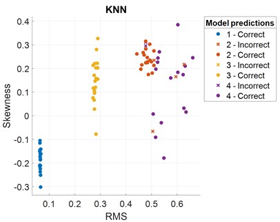
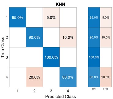
Fig. 7Scatter plot and confusion matrix for KNN classifier with the feature set 3
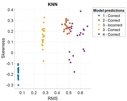
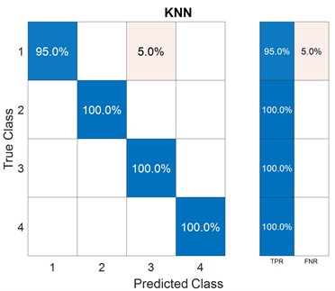
Table 2Selected features and associated fault classification accuracies of SVM and KNN classifiers
Feature set | Features | Classifier | Accuracy |
Set 1: Combination of time and frequency-domain features | Crest factor, impulse factor, kurtosis, RMS, SNR, skewness, peak amplitude, peak frequency, Lyapunov exponent | SVM | 95.0 % |
KNN | 96.2 % | ||
Set 2: Non-linear time-domain features | Approximate entropy, correlation dimension, Lyapunov exponent | SVM | 88.8 % |
KNN | 91.2 % | ||
Set 3: Frequency-domain features | Peak amplitude, peak frequency, band power | SVM | 96.2 % |
KNN | 98.8 % |
5. Conclusions
The current research, which employs machine learning techniques, demonstrates that the specific selection of fault features plays a significant role in training machine learning models for bearing defect classification. The set of frequency-domain features has the best performance in both SVM and KNN classifiers among the three feature sets. The fault classification accuracy is the lowest when just non-linear time-domain features are used for ML model training. However, the accuracy increases significantly with a combination of features from time-domain and frequency-domain. With only frequency-domain features, the accuracy further improves. This trend can be observed in both the SVM and the KNN classifiers. Also, in all three cases, KNN outperforms SVM. As a result, frequency-domain is more supportive in identifying rolling element bearing defects in terms of fault features, and the KNN model beats the SVM model.
References
-
A. Widodo et al., “Fault diagnosis of low speed bearing based on relevance vector machine and support vector machine,” Expert Systems with Applications, Vol. 36, No. 3, pp. 7252–7261, Apr. 2009, https://doi.org/10.1016/j.eswa.2008.09.033
-
P. S. Bhowmik, S. Pradhan, and M. Prakash, “Fault diagnostic and monitoring methods of induction motor: a review,” International Journal of Applied Control, Electrical and Electronics Engineering, Vol. 1, No. 1, pp. 1–18, 2013.
-
M. Orman, P. Rzeszucinski, A. Tkaczyk, K. Krishnamoorthi, C. T. Pinto, and M. Sulowicz, “Bearing fault detection with the use of acoustic signals recorded by a hand-held mobile phone,” in 2015 International Conference on Condition Assessment Techniques in Electrical Systems (CATCON), pp. 252–256, Dec. 2015, https://doi.org/10.1109/catcon.2015.7449545
-
S. Khanam, N. Tandon, and J. K. Dutt, “Fault size estimation in the outer race of ball bearing using discrete wavelet transform of the vibration signal,” Procedia Technology, Vol. 14, pp. 12–19, 2014, https://doi.org/10.1016/j.protcy.2014.08.003
-
R. B. Randall and J. Antoni, “Rolling element bearing diagnostics-A tutorial,” Mechanical Systems and Signal Processing, Vol. 25, No. 2, pp. 485–520, Feb. 2011, https://doi.org/10.1016/j.ymssp.2010.07.017
-
O. Janssens et al., “Thermal image based fault diagnosis for rotating machinery,” Infrared Physics and Technology, Vol. 73, pp. 78–87, Nov. 2015, https://doi.org/10.1016/j.infrared.2015.09.004
-
K. C. Deekshit Kompella, M. V. G. Rao, R. S. Rao, and R. N. Sreenivasu, “Estimation of nascent stage bearing faults of induction motor by stator current signature using adaptive signal processing,” in 2013 Annual IEEE India Conference (INDICON), pp. 1–5, Dec. 2013, https://doi.org/10.1109/indcon.2013.6725956
-
B. Li, M. Y. Chow, Y. Tipsuwan, and J. C. Hung, “Neural-network-based motor rolling bearing fault diagnosis,” IEEE Transactions on Industrial Electronics, Vol. 47, No. 5, pp. 1060–1069, 2000.
-
M. A. Jamil and S. Khanam, “Multi-class fault classification of rolling element bearing in machine learning environment,” in International Conference on Condition Monitoring, Diagnosis and Maintenance, 2021.
-
H. Ocak and K. A. Loparo, “A new bearing fault detection and diagnosis scheme based on hidden Markov modeling of vibration signals,” in 2001 IEEE International Conference on Acoustics, Speech, and Signal Processing. Proceedings, Vol. 5, pp. 3141–3144, 2001, https://doi.org/10.1109/icassp.2001.940324
-
P. D. McFadden and J. D. Smith, “Vibration monitoring of rolling element bearings by the high-frequency resonance technique – a review,” Tribology International, Vol. 17, No. 1, pp. 3–10, Feb. 1984, https://doi.org/10.1016/0301-679x(84)90076-8
-
C. Cortes and V. Vapnik, “Support-vector networks,” Machine Learning, Vol. 20, No. 3, pp. 273–297, Sep. 1995, https://doi.org/10.1007/bf00994018
-
M. J. Hasan, J. Kim, C. H. Kim, and J.-M. Kim, “Health state classification of a spherical tank using a hybrid bag of features and K-nearest neighbor,” Applied Sciences, Vol. 10, No. 7, p. 2525, Apr. 2020, https://doi.org/10.3390/app10072525
-
J. Tian, C. Morillo, M. H. Azarian, and M. Pecht, “Motor bearing fault detection using spectral kurtosis based feature extraction and k-nearest neighbor distance analysis,” IEEE Transactions on Industrial Electronics, Vol. 63, No. 3, pp. 1793–1803, Mar. 2016, https://doi.org/10.1109/tie.2015.2509913
-
L. Greche, M. Jazouli, N. Es-Sbai, A. Majda, and A. Zarghili, “Comparison between Euclidean and Manhattan distance measure for facial expressions classification,” in 2017 International Conference on Wireless Technologies, Embedded and Intelligent Systems (WITS), pp. 1–4, Apr. 2017, https://doi.org/10.1109/wits.2017.7934618
-
“Bearing Data Center.” Case Western Reserve University. https://csegroups.case.edu/bearingdatacenter/pages/welcome-case-western-reserve-university-bearing-data-center-website
