Bearing fault diagnosis method based on Gramian angular field and ensemble deep learning

1. Introduction

In modern industries, machine health monitoring is a prerequisite for maintaining the proper operation of industrial machines. Breakdowns in industrial machines can cause huge financial losses and even pose a threat to the people who use them. Therefore, the need for better and smarter machine health-monitoring technologies has never ceased [1]. Rolling bearings are considered the most common and critical mechanical components in rotating machinery, and their health can have a significant impact on the performance, stability, and service life of the machine. Because rolling bearings are usually in harsh operating environments, they are prone to failure during operation. Failure to detect defects in time can lead to unplanned machine downtime or even catastrophic damage. Therefore, rolling bearing fault detection is essential for the safe and reliable operation of machinery and production [2].

Recently, several bearing fault recognition methods have been proposed. Learning-based (including statistical learning methods and neural network methods) recognition methods can capture mechanical fault information by learning historical data and thereby enabling the automated analysis of bearing faults. The flow chart of these methods usually includes data preprocessing, feature extraction, and classifier design. Although a well-designed classification algorithm is a prerequisite for automated bearing fault detection [3], data preprocessing and feature extraction are also important steps.

Designing manual features based on the signal mechanism is a hot field for bearing fault diagnosis. Chen et al. [4] merged the bearing signal features of the time and frequency domains and then inputted these features into a deep fully connected network for fault detection. Bao et al. [5] calculated the L-kurtosis feature in the envelope spectrum of a vibration signal to detect pulse periodicity. Chen et al. [6] first transformed a vibration signal into the spectrum domain and extracted the mapping amplitude entropy as a learnable feature. Zhao et al. [7] first performed empirical mode decomposition (EMD) on a vibration signal, and then selected the top few-mode components containing the main information of the signal to extract the sample entropy. Liu et al. [8] proposed a feature extraction method based on variational mode decomposition and singular value decomposition (SVD). Unfortunately, these manual feature extraction processes are laborious and unfriendly to machine-learning designers.

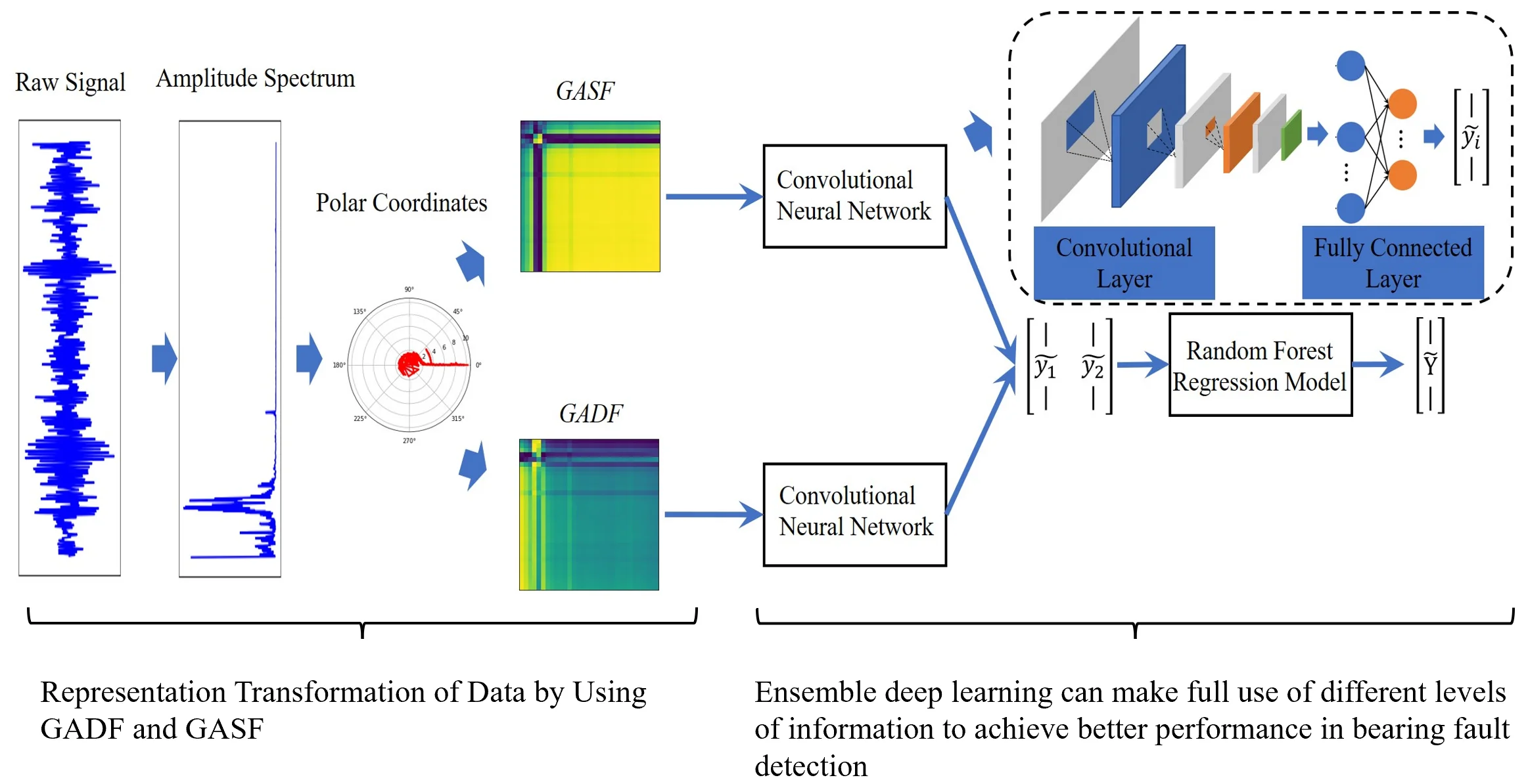
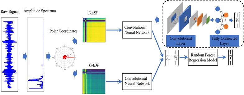
Fig. 1The flow chart of the proposed method

Owing to the powerful feature learning ability of deep learning techniques, many researchers have attempted to introduce deep learning into the field of fault detection. Example include convolutional neural network (CNN)-based methods [1], [2], [9], [10]-[14], sparse auto-encoder (SAE)-based methods [15], [16], and recursive neural network (RNN)-based methods [17], [18], etc. Because the original signal is easily affected by noise, the signal is often transformed into an amplitude-frequency domain sequence. Generally speaking, CNN models are good at learning deep features from image data; thus, one-dimensional vibration signals encoded as two-dimensional image data have attracted much attention. CNN and their improved models have been successfully applied to image classification because they can extract robust features directly from two-dimensional images. Many image-interpreting vibration signal approaches have been proposed. Ding et al. [2] proposed a method for reconstructing a two-dimensional wavelet packet energy image (WPI) of the frequency space. The WPI can represent the dynamic structure of the wavelet packet energy distribution of different bearing faults. However, the WPI method combines the wavelet packet transform and phase space reconstruction technique, which not only has high time complexity but also loses the information of the original signal when performing multiple transformations of the representation space. Mantas et al. [19] converted the time series to the Permutation Entropy (PE) pattern, which is a 2D digital image with multiscale time delays. However, the method ignores the amplitude information of the time series, and it is sensitive to noise in the view of the principle behind the method. Wang et al. [20] combined Symmetrized Dot Pattern (SDP) with CNN for intelligent bearing fault diagnosis. SDP method [21] converts the time series into polar SDP images, which have the frequency and amplitude of the raw signals. In [22] and [9], they convert the time series into a 2D gray image. In addition, a variety of methods use the time-frequency image to represent the time series [23], [24], but the time-frequency analysis methods cost a lot of time so it is difficult for actual online diagnosis. Wang et al. [25] encoded a time series as the GAF image and then took advantage of the deep model for image representation learning to obtain a better classification accuracy rate. The algorithm was validated on a 20-time series dataset and outperformed the traditional k-NN+DTW method, which was earlier considered the most effective method for time series classification.

The advantages of image-interpreting time series as a GAF image include the following: 1) there is no spatial transformation of the original time series, and the encoding process is performed in the original representation space. In other words, the time complexity of the algorithm is of the linear order Ο($n$), where n is the length of the time series. 2) The principle of the approach is simple, easy to understand, and reproducible. Surprisingly, the GAF pictorial method has rarely been applied to bearing fault detection problems. The GAF pictorial method has two different representations, including the Gramian Angular Summation Field (GASF) and the Differential Difference Field (GADF). The GASF and GADF provide different levels of information, such that, the final decision results of using them for deep learning are different. Given this, this study introduces the stacking generalization method [26], [27] to fuse the initial decision results based on GASF and GADF. The proposed method improved the classification accuracy rate of bearing faults and increased the reliability of the results.

The flow of the proposed approach is shown in Fig. 1. It can be seen that the method is composed of data preprocessing, image-interpreted vibration signal, and ensemble deep learning. The image-interpreting stage was used to better explore the vibration signals information. Ensemble deep learning can make full use of different levels of information to achieve better performance in bearing fault detection.

In sum, the main contributions of this study are as follows:

1) The GAFs approach is introduced to encode the bearing vibration signal into GASF and GADF matrices. The GAFs contain temporal correlation of vibration signal. The 2D-CNN is used to learn the deep features of the images, and then the idea of the stacking ensemble method is combined to construct an integrated deep model to achieve a high accuracy rate of bearing fault detection. It is a decision-level fusion strategy. Due to the deep learning with GASF and GADF obtains different accuracy rates, namely, they contain different information for classification. Therefore, building an ensemble model is an ideal fault detection scheme.

2) Last but not least, we design two experiments on CWRU datasets to evaluate the performance of bearing fault classification. With those comparable results, we demonstrate that our method achieves a better performance than the comparative method.

3) The rest of the paper is organized as follows: In Section 2, we introduce the principle of encoding time series as GAF images; we present the proposed method in Section 3; next, we conduct a performance test on the CWRU dataset. Finally, in Section 5, we conclude the paper.

2. Image-interpreted time series

Encoding vibration signals into images of different granularities is a popular research area for bearing fault diagnosis. Here, we introduce the GAF encoding method, which first transforms the vibrating bearing signal into a 2D image, and then uses a 2D-CNN to learn the knowledge of the image.

2.1. GAF encoding method

Given a time series $X=\left\{x_1,x_2,\cdots ,x_n\right\}$, where $x_i$ is scaled in $[-\mathrm{1,1}]$ or $\left[\mathrm{0,1}\right]$ using:

1

$\widetilde{x_i}=\frac{x_i-max\left(X\right)+x_i-min\left(X\right)}{max\left(X\right)-min\left(X\right)},$

2

$\widetilde{x_i}=\frac{x_i-min\left(X\right)}{max\left(X\right)-min\left(X\right)}.$

Then, the $\tilde{X}$ can be encoded as the angular cosine and the timestamp as the radius using Eq. (3):

3

$\left\{\begin{array}{ll}\varphi =\mathrm{a}\mathrm{r}\mathrm{c}\mathrm{c}\mathrm{o}\mathrm{s}\left(\widetilde{x_i}\right),& -1\le \widetilde{x_i}\le 1,\mathrm{}\mathrm{}\mathrm{}\mathrm{}\widetilde{x_i}\in \widehat{\mathit{X}},\\ r=\frac{t_i}{N},& t_i\in \mathbb{N},\end{array}\right.$

where $t_i$ is the timestamp and $N$ is a constant factor. Based on this, a one-dimensional time series is mapped to the two-dimensional image. Because $x_i\in \left[-\mathrm{1,1}\right]$ or $x_i\in \left[\mathrm{0,1}\right]$, $\mathrm{c}\mathrm{o}\mathrm{s}\left(\varphi \right)$ ($\varphi \in \left[0,\pi \right]$) is monotonic, such that GAF encoding is bijective. In other words, a time series can be mapped only to a unique polar coordinate space. In addition, the time dependence is preserved by the $r$ coordinates.

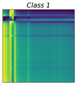
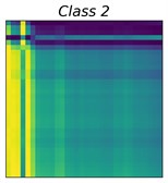
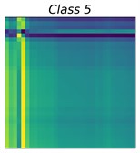
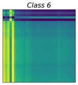
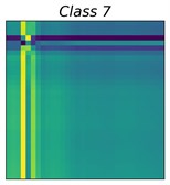
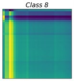
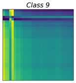
Fig. 2GASF images of 10 bearing status

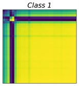
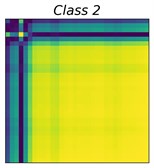
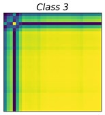
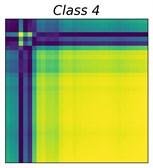
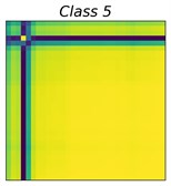
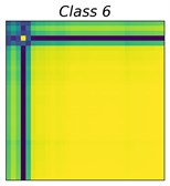
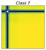
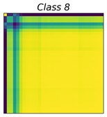
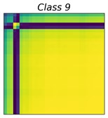
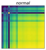
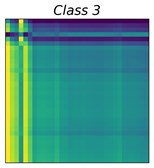
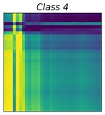
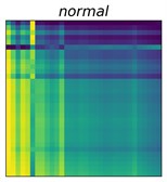
Fig. 3GADF images of 10 bearing status

Once performing the GAF encoding for time series, the temporal correlations within different time intervals are identified by considering the triangular sum/difference between each point:

4

$GASF\left(i,j\right)=\mathrm{c}\mathrm{o}\mathrm{s}\left({\varphi }_i+{\varphi }_j\right)=\widetilde{x_i}\widetilde{x_j}-\sqrt{1-{\left(\widetilde{x_i}\right)}^2}\sqrt{1-{\left(\widetilde{x_j}\right)}^2},$

5

$GADF\left(i,j\right)=\mathrm{s}\mathrm{i}\mathrm{n}\left({\varphi }_i-{\varphi }_j\right)=\widetilde{x_j}\sqrt{1-{\left(\widetilde{x_i}\right)}^2}-\widetilde{x_i}\sqrt{1-{\left(\widetilde{x_j}\right)}^2}.$

The GAF matrix was constructed in the original representation space of the time series. Therefore, the encoding method has significant advantages in terms of efficiency, while avoiding temporal information loss in the process of representation space transformation [25]. Work [25] pointed out that the GAF has two significant advantages. First, the GAF matrix preserves the time dependence of the time series, that is, each element of the GAF matrix was generated sequentially from the top left to the bottom right according to the temporal order of the original time series. Second, the GAF matrix contains temporal correlations; for example, $GAF\left(i,j\right)$ denotes the time interval $k=\left|i-j\right|$ relative correlation in the direction.

In practical applications, direct encoding of the bearing vibration signal in the time domain into a GAF matrix is often unsatisfactory. This is because the bearing signal in the time domain can easily be contaminated by noise. Therefore, we encoded the amplitude-spectrum sequence of the bearing signal into the GAF image. In the amplitude spectrum, the energy of useful information is concentrated in a narrow range of frequency bands, whereas the noise energy is distributed over the entire frequency band. Assuming that $\stackrel{-}{X}=\left\{\stackrel{-}{x_1},\stackrel{-}{x_2},\cdots ,\stackrel{-}{x_n}\right\}$ is the amplitude spectrum of a bearing vibration signal, such that $\stackrel{-}{X}$ can be denoised according to Eq. (6):

6

${\left(\stackrel{-}{x_i}\right)}^{\mathrm{\text{'}}}=\left\{\begin{array}{c}\stackrel{-}{x_i}-\mu ,\stackrel{-}{x_i}>\mu ,\\ 0,\stackrel{-}{x_i}\le \mu ,\end{array}\right.$

where, $\mu$ is the mean value of $X$. As the amplitude spectrum of the vibration signal is symmetric, it is possible to consider only the left amplitude spectrum. Fig. 2 and 3 show the GASF and GADF images of 10 different bearing faults, respectively. The class distributions of these faults are shown in Table 1.

Table 1Class distribution of 9 types of faults

Fault type	Load (HP)	Speed (rpm)	Ball	Inner race	Outer race
0.007"	0	1797	class 1	class 4	class 7
0.014"	0	1797	class 2	class 5	class 8
0.021"	0	1797	class 3	class 6	class 9

3. Denoising method

In real applications, the sampling points of the time series are usually very large; therefore, it is necessary to reduce the dimensionality of the time series before GAF encoding. Considering that the piecewise aggregate approximation (PAA) algorithm [28] can not only preserve the basic trend of the time series but also has low time complexity, we use the PAA algorithm to pre-process the bearing vibration signal.

PAA is a simple and effective time series smoothing algorithm that preserves the trend of the time series. The time complexity of PAA is low; therefore, the PAA algorithm is widely used in time series analysis problems. Considering the time series $X=\left\{x_1,x_2,\cdots ,x_n\right\}$ is mapped to a new time series $\widehat{X}=\left\{\widehat{x_1},\widehat{x_2},\cdots ,\widehat{x_m}\right\}$,$\mathrm{}\widehat{x_i}$ can be calculated using the following formula:

From Eq. (7), we find that $X$ is sequentially divided into $m$ blocks of equal size, and the mean value of each block is used to re-represent the block. The PAA algorithm has a certain noise reduction effect, as it uses the mean value to smooth the data. Clearly, the selection of $m$ is crucial. If $m$ is too large, the smoothed result loses the original structural information, where $m$ is too small, and the effect is not suitable for noise reduction. From Eq. (7), we can also see that the traditional PAA needs to satisfy $n/m$ as an integer. For $n/m$ is a non-integer number that can be found in [29] and [30].

4. Experiments

Here, we used CWRU bearing data [36] to verify the effectiveness of the proposed method. The dataset comprised a multivariate vibration time series generated by the bearing test equipment, as shown in Fig. 4. In this study, the bearing dataset included the following four conditions: normal, outer race failure, inner race failure, and roller failure. The drive-side vibration signal was used with a sampling rate of 48 kHz and a motor load of 0 hp. Table 1 shows the class distributions of the selected data.

Fig. 4Test-stand [36]

5. Experimental design

Here, we used a 2D-CNN as the initial learner. Considering useable data is small, the 2D-CNN model includes only three convolutional layers, three pooling layers, and one fully connected structure. Meanwhile, the batch normalization [37] and the dropout [38] methods are used to reduce the risk of deep model over-fitting. The 2D-CNN uses the cross-entropy loss function, and Adam optimizes the algorithm [39]. We used the random forest regression method as the meta-learner. We follow the common practice of dividing the CWRU dataset was divided into the training set, test set, and validation set in the ratio of 0.5, 0.3, and 0.2. The training set was used to train the 2D-CNN and the validation set was used to train the random regression model. The experiments are repeated 10 times under different random seeds, and the final results are taken as the mean value of the 10 experiments. Considering the uniform distribution of classes, performing different algorithms can be well measured by the traditional classification accurate rate:

6. Conclusions

This study proposed a bearing fault detection method that combines im-age-interpreting vibration signals and integrating deep learning, which can realize the accurate identification of bearing faults. Our method encoded one-dimensional vibration signals into a two-dimensional image and then used a 2D-CNN to obtain the initial decision result. Finally, we introduced a decision layer integration method to realize the fusion of multiple underlying decisions. Experiments on the CWRU real-world dataset show that the proposed method can obtain a better recognition accuracy rate than the existing method (i.e., WPI+2D-CNN), even when Gaussian white noise is added to the original vibration signal.

Altogether, the learning-based method for bearing fault detection is provided in this work. Next, we plan to apply our method to different publicly available bearing failure datasets and laboratory datasets.