Enhancing non-destructive testing in concrete structures: a GADF-CNN approach for defect detection

2.1. Gramian angular difference field

The GADF is a transformation technique that encodes time-series data into a 2D representation. The GADF is derived from the Gramian Angular Field (GAF), which is computed by mapping the time-series data into a polar coordinate system. The GAF is then computed as the outer product of the transformed data with itself.

To not bias the inner product towards the maximum observations, the time series $X=\{x_1,x_2,\cdots ,x_n\}$ is scaled into the interval [–1, 1]. This can be achieved by applying the following transformation:

where $X\text{'}$ is the scaled time series, $\mathrm{m}\mathrm{i}\mathrm{n}\left(X\right)$ and $\mathrm{m}\mathrm{a}\mathrm{x}\left(X\right)$ are the minimum and maximum values of the time series, respectively.

The scaled time series is then converted to polar coordinates. The radial coordinate $r$ is computed as the absolute value of the scaled time series $X\text{'}$, and the angular coordinate $\theta$ is computed as:

The GAF is computed as the outer product of the angular coordinates with themselves:

where $\otimes$ denotes the outer product operation.

The Gramian Angular Summation Field (GASF) and the GADF are both image transformation techniques that convert one-dimensional time series data into two-dimensional images. While GASF captures temporal correlations by using the sum of the phase space, GADF emphasizes changes in the data by using the difference of the phase space. The GASF and GADF can be computed using the following equations:

where ${\theta }_i$ and ${\theta }_j$ are the angular coordinates of the $i$th and $j$th data points, $GASF(i,j)$ and $GADF(i,j)$ are the elements of the GASF and GADF, respectively.

In certain scenarios, the GADF demonstrates superior performance over the GASF, attributable to its emphasis on data variation. This attribute is particularly beneficial in applications where change detection is critical, such as in the identification of defects in concrete structures. Consequently, the GADF technique has been utilized in this research. It effectively converts time-series data into a two-dimensional format, thereby augmenting the model's capacity to discern and assimilate these pivotal variations.

2.2. The CNN depth network

A CNN is composed of several types of layers, each performing a specific operation on the input data. These layers include convolutional layers, pooling layers, fully connected layers, and a classifier layer [35], [36].

Convolutional layers apply a set of learnable filters to the input data. Each filter is convolved across the width and height of the input to produce a feature map. This operation can be represented mathematically as:

where $Y_{l-1,i+m,j+n}$ is the input from the $\left(l-1\right)$th layer at location $\left(i+m,j+n\right)$, $W_{l,m,n}$ and $b$ are the weights and bias of the $l$th layer, $*$ is the convolution operation, $Y_{l,i,j}$ is the output of the $l$th layer at location $\left(i,j\right)$, $f_l$ is the activation function of the $l$th layer.

Pooling layers reduce the spatial dimensions of the input, typically using a max or average operation. This operation can be represented mathematically as:

where $P$ is the pooling region.

Fully connected layers, also known as dense layers, connect every neuron in the layer to every neuron in the previous layer. This operation can be represented mathematically as:

where $Y_{l,i}$ is the input from $\left(l-1\right)$th layer, $W_{l,i,j}$ and $b_{l,i}$ are the weights and bias of the $l$th layer, $Y_{l,i}$ is the output of the $l$th layer at location $i$, $f_l$ is the activation function of the $l$th layer.

The final layer of the CNN is typically a classifier layer that uses a SoftMax function to output a probability distribution over the classes. This operation can be represented mathematically as:

where $Y_{L-1,i}$ is the input from the $\left(L-1\right)$th layer, $Y_{L,i}$ is the output of the $L$th layer (classifier layer) at location $i$.

2.3. Depthwise separable convolution and attention mechanisms

In the quest to improve the performance of our CNN model for concrete structure defect recognition, we incorporate two advanced concepts: Depthwise Separable Convolution and Attention Mechanisms. These techniques are aimed at enhancing the model's ability to learn more complex and abstract features from the GADF-transformed data, while also improving computational efficiency.

Depthwise Separable Convolution is a variant of the standard convolution operation that is used in traditional CNN. It involves two separate operations: a depthwise convolution followed by a pointwise convolution. This operation can be represented mathematically as:

where $Y_{l-1,i+m,j+n}$ is the input from the $\left(l-1\right)$th layer at location $(i+m,j+n)$, $W_{l,m,n}$ and $b_l$ are the weights and bias of the $l$th layer, $\cdot$ is the convolution operation, $Y_{l,i,j}$ is the output of the $l$th layer at location $(i,j)$, $f_l$ is the activation function of the $l$th layer. The depthwise convolution applies a single filter to each input channel.

The pointwise convolution then applies a 1×1 convolution to combine the outputs of the depthwise convolution. This operation reduces the computational cost and model size compared to standard convolutions, making the model more efficient and faster to train.

Attention Mechanisms, on the other hand, allow the model to focus on the most relevant parts of the input for making predictions. In the context of our task, this means that the model can learn to pay more attention to the parts of the GADF-transformed data that are most indicative of a defect in the concrete structure.

The attention mechanism can be represented mathematically as:

where $Y_{l-1,j}$ is the input from the $\left(l-1\right)$th layer, $W_{l,i,j}$ and $b_{l,i}$ are the weights and bias of the $l$th layer, $Y_{l,i}$ is the output of the $l$th layer at location $i$, $f_l$ is the activation function of the $l$th layer.

The use of Depthwise Separable Convolution and Attention Mechanisms in the CNN depth network enhances the network's ability to recognize defects in concrete structures. This dual incorporation not only enhances the model's ability to learn complex and abstract features from the GADF-transformed data, but also improves computational efficiency, making it a powerful tool for concrete structure defect recognition.

2.4. Developing methodology for concrete structure defect recognition

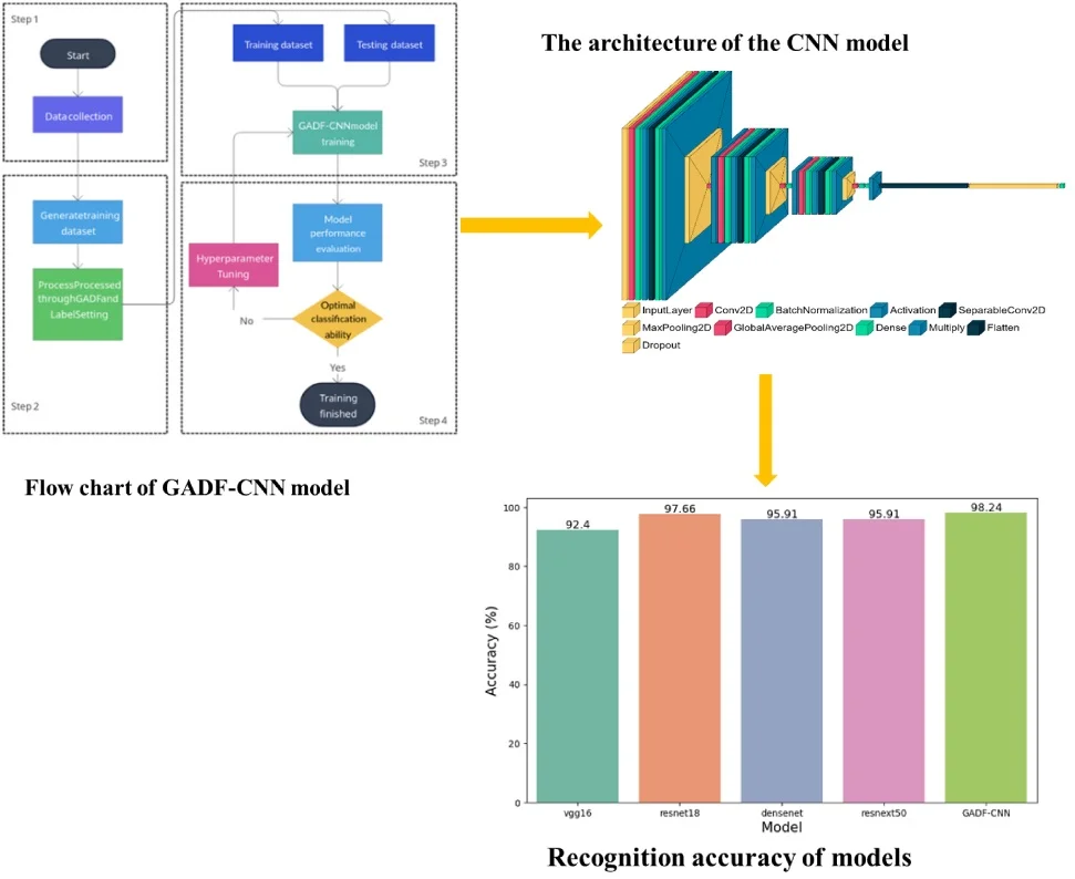
In the development of a comprehensive methodology for concrete structure defect recognition, the integration of the GADF and the CNN depth network, enhanced with Depthwise Separable Convolution and Attention Mechanisms, is crucial. This section outlines the process of integrating these components into a cohesive methodology (Fig. 1).

Fig. 1Methodology for concrete structure defect recognition

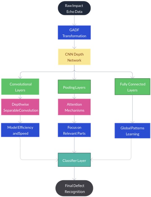
The first step in our methodology is the application of the GADF transformation to the raw impact echo data. This transformation, as detailed in Section 2.1, encodes the time-series data into a 2D representation. The GADF transformation serves to enhance the spatial-temporal features of the data, effectively converting the impact echo data into an image-like format. This conversion is a critical step as it allows the subsequent CNN to process the data effectively.

Once the data has been transformed using the GADF, it is input into the CNN depth network. The CNN, as discussed in Section 2.2, consists of several layers, each performing a specific operation on the input data. The convolutional layers apply a set of learnable filters across the width and height of the input data, producing a feature map. The pooling layers reduce the spatial dimensions of the data, summarizing the extracted features over spatial regions. The fully connected layers connect every neuron in one layer to every neuron in the previous layer, learning global patterns in the data. The classifier layer outputs a probability distribution over the classes, providing the final defect recognition results.

To optimize the performance and efficiency of the CNN model, this study integrates Depthwise Separable Convolution and Attention Mechanisms, as detailed in Section 2.3. Depthwise Separable Convolution minimizes computational demands and model dimensions, thus enhancing efficiency and expediting the training process. Conversely, Attention Mechanisms enable the model to concentrate on the most salient segments of the input for prediction purposes. The model is trained to prioritize areas in the GADF-transformed data that most strongly indicate defects in concrete structures.

For the computational implementation, Python version 3.8 and PyTorch were utilized to develop and test the neural networks, providing a robust framework for the efficient execution of large-scale numerical computations. For benchmarking, the model's performance was evaluated against established methods using the Impact Echo dataset, recognized for its relevance in the field of non-destructive testing in concrete structures. The experimental design for the Impact Echo dataset is detailed in Section 3.

Summarily, the integration of the GADF transformation, the CNN depth network, and the Depthwise Separable Convolution and Attention Mechanisms forms the basis of the methodology for concrete structure defect recognition. This integration leverages the strengths of each component, resulting in a powerful model capable of accurately recognizing defects in concrete structures.

3.1. Collection of impact echo data

The experimental setup began with the creation of multiple concrete slabs, each incorporating a range of potential defects. In a controlled laboratory setting, two concrete model specimens were fabricated, designed to simulate four distinct internal defect scenarios: intact structure, non-compact areas, voids, and water-filled voids. Each model was constructed with dimensions of 150 cm in height, 220 cm in length, and a variable thickness of 60 to 70 cm. Hollow cylinders with a diameter of 20 cm were embedded in the specimens to replicate void defects. These cylinders were either left vacant to represent air voids or filled with water to simulate water-filled voids. For non-compact defect emulation, the cylinders were filled with loosely packed materials. The defects were strategically placed at varying depths (10 cm, 20 cm, 30 cm, and 40 cm) within the specimens to accurately represent possible real-world defect scenarios. Detailed visual documentation of the construction process of these models is presented in Fig. 2.

The next phase of the research involved acquiring impact echo data. The equipment for these tests, including a steel ball array, a handheld transducer, a data acquisition (DAQ) system, and a computer with specialized analytical software, was sourced from IEI, LLC in Ithaca, NY, USA. Precise adjustment of signal sampling frequency and length was crucial for the success of the impact-echo tests. These parameters were instrumental in accurately capturing the impact-echo signal with maximum response frequency, thereby ensuring optimal sampling resolution. Guided by the physical properties of the specimens, the sampling frequency was set at 500 kHz and the sampling length at 1024. The testing process entailed generating stress waves by striking the concrete surface with an impactor, followed by using a sensor to record the reflected waves. This procedure was systematically repeated across various points on the concrete structure to amass a comprehensive dataset. This approach yielded a total of 830 samples, each categorized into one of the four predefined internal defect types: sound, non-compact, voids, and water-filled [18].

Following the data collection, the data undergoes several preprocessing steps. These steps are integral to the process and include normalization, and segmentation.

Normalization ensures that the data is in a suitable format for the subsequent steps. This is done by scaling the data to have a zero mean and unit variance, which can be represented as:

where $\mu$ and $\sigma$ are the mean and standard deviation of the noise-reduced data, respectively, $X\text{'}\text{'}\left(t\right)$ is the normalized data.

Fig. 2Preparation of experimental concrete slabs: a) constructing the concrete specimen mold; b) the concrete slab specimens after they have been poured

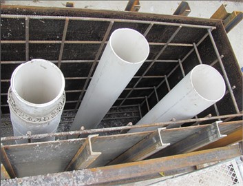
a)

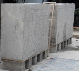
b)

Segmentation divides the data into manageable chunks that can be processed individually. This can be represented as:

where $i$ is the segment index, $T$ is the segment length, $X_i\left(t\right)$ is the $i$th segment of the normalized data. The collected impact echo data will serve as the input for our CNN model after preprocessing steps.

3.2. Design for implementing CNN with depthwise separable convolutions and attention mechanisms

A pivotal aspect of the experimental design is the deployment of a CNN integrated with Depthwise Separable Convolutions and Attention Mechanisms. The CNN is engineered to process the impact echo data, which is transformed into a two-dimensional format using the GADF. The architecture of the CNN encompasses various layers: convolutional layers augmented with Depthwise Separable Convolutions, pooling layers complemented by Attention Mechanisms, fully connected layers, and a classifier layer, as depicted in Fig. 3. The construction of the CNN adheres to the principles delineated in the methodology section (Section 2).

Fig. 3The architecture of CNN with depthwise separable convolutions and attention mechanisms

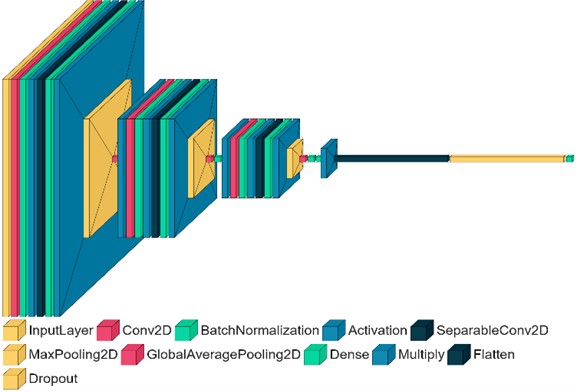
The model architecture is composed of a sequence of layers that sequentially process the input data. Initially, a series of DepthwiseSeparableConv layers are applied, each of which is followed by batch normalization, a ReLU activation function, and max pooling. These layers are primarily responsible for feature extraction from the input data. Subsequently, an AttentionModule is incorporated after each max pooling layer. These modules enhance the model's capability to focus on the most relevant features. To prevent overfitting during the training phase, a dropout layer is included, which randomly sets a fraction of input units to zero at each update. Finally, a fully connected (Linear) layer is employed to transform the extracted features into a set of class scores, completing the model architecture. Table 1 summarize the parameter settings of each layer in the model architecture:

In the machine learning model's training process, each category's samples are divided into three parts (the training set, the validation set, and the testing set) according to the ratio of 4:1:1. The defect samples included: 1200 sound samples, 1200 non-compact samples, 1200 voids samples, and 1200 water-filled samples. The dataset is shown in Table 2.

Fig. 4Flow chart of GADF-CNN model training and application

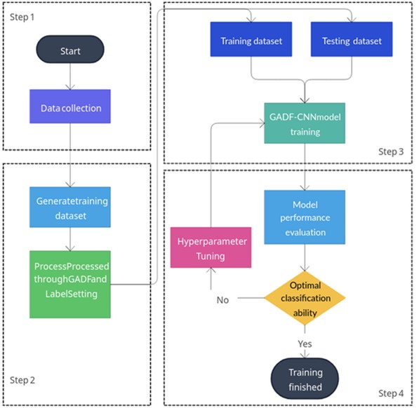
The concrete defect classification steps based on GADF-CNN are shown in Fig. 4. The specific steps are as follows:

1) Use the impact echo instrument to detect different types of concrete structures with defects on-site, collect the impact echo vibration signals to form the original dataset for the model, and preprocess the raw data.

2) Process the preprocessed raw dataset with GADF and label it to generate the sample set for the model.

3) To train the GADF-CNN model, randomly sample all sets of data and divide them into training and test sets in an 8:2 ratio. Feed these sets to the model to complete the training process. Save the weight file when the classification accuracy reaches its highest point during the training process.

4 After the model training is completed, adjust the model's hyperparameters based on its performance on the test set, and retrain the GADF-CNN model until it performs best on the test set, i.e., the model reaches the ideal state.

The following pseudo-code provides a detailed description of the GADF-CNN Processing Algorithm, highlighting its key components and operations.

4.1. Presentation of the results

In the evaluation of the proposed methodology, several metrics were used to assess the model's performance. These include the accuracy rate (Acc), recall rate (Rec), F1 score (F1), and confusion matrix (CM).

The accuracy rate (Acc) is a measure of the proportion of total predictions that are correct. It is calculated using the formula:

where TP is the number of true positives, TN is the number of true negatives, FP is the number of false positives, FN is the number of false negatives.

The recall rate (Rec), also known as sensitivity or true positive rate, is the proportion of actual positive cases that were correctly identified. It is calculated as:

The F1 score (F1) is the harmonic mean of precision and recall, providing a balance between these two metrics. It is calculated as:

where Precision is the proportion of positive identifications that were actually correct, calculated as:

The confusion matrix (CM) is a robust tool for evaluating classification model performance, providing a detailed breakdown of correct and incorrect predictions across different classes. It organizes predictions into a tabular format, with rows representing predicted classes and columns denoting actual classes. Correct predictions populate the matrix’s diagonal, while off-diagonal elements signify errors. Through a comprehensive analysis of the CM, one can discern the error types prevalent in the classifier's performance, thereby illuminating potential avenues for model improvement.

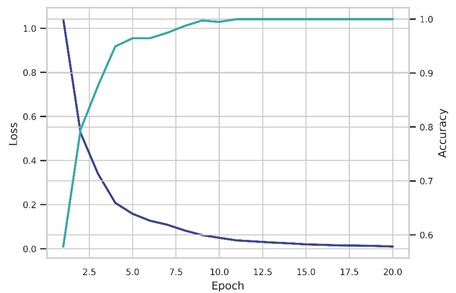
Throughout the model training process, performance metrics were evaluated on a training dataset at the completion of each epoch. The training utilized a batch size of 32, allowing for efficient processing and model weight updates. The Adam optimizer, with a learning rate of 0.0001, facilitated gradual and stable improvements in model performance. To prevent overfitting, a regularization strategy involving a dropout rate of 0.5 was applied within the classifier. This approach was chosen based on its proven effectiveness in enhancing generalizability while maintaining model simplicity.

As training progressed over 20 epochs, the model demonstrated improved accuracy and reduced loss, as depicted in Fig. 5. This iterative process allowed for continuous refinement of the model’s weights, ensuring that each epoch contributed to the model's ability to discern intricate patterns within the dataset. The training was implemented on a T4 GPU and took 30.748 seconds, further supporting that the proposed model is a less resource-intensive method for concrete structure defect recognition. The combination of strategic parameter selection and advanced hardware utilization underscores the model's efficiency and effectiveness in identifying defects within concrete structures.

Fig. 5Illustration of loss value and accuracy curves over time

The final performance of the model on the testing set for each of the four categories of concrete defects is summarized in Table 4.

Table 4 presents the performance metrics of the proposed model for four categories of concrete defects. The model exhibits high precision, recall, and F1 scores across all categories, indicating its effectiveness in accurately identifying and classifying defects. For instance, the “Sound” category achieved a precision of 0.9607 and a perfect recall of 1.0000. The “Non-compact” category achieved perfect scores across all metrics. Despite slightly lower recall rates in the 'Voids' and “Water filled” categories, the overall accuracy of the model remains high, affirming the model's robustness in concrete structure defect recognition.

The corresponding confusion matrix for the model’s predictions on the testing set is provided in Fig. 6.

Fig. 6The confusion matrix of four category’s internal defects

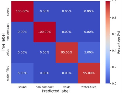
The confusion matrix offers a visual insight into the model’s performance. Each row signifies the instances in a predicted class, while each column represents the instances in an actual class. The diagonal elements indicate correct predictions, while off-diagonal elements represent misclassifications. The matrix reveals a high degree of accuracy, with most misclassifications occurring between the “Voids” and “Water filled” categories.

4.2. Evaluation of statistical indicators

Evaluating the performance and reliability of the GADF-CNN approach for defect detection necessitates a comprehensive assessment of statistical indicators such as uncertainty, sensitivity, and confidence intervals. These metrics are essential for understanding the limitations and potential issues related to the model's measurements, which can be influenced by factors like input data noise, defect characteristic variations, and model architecture limitations. Sensitivity analysis identifies the impact of these factors on the model's outputs, while confidence intervals provide a statistical range for the true performance metrics, considering the inherent variability in the measurements.

Monte Carlo Dropout (MCD) is a technique for estimating prediction uncertainty in CNN models. It involves performing multiple forward passes through the network with dropout enabled during inference. The dropout layers randomly set a fraction of the neurons to zero, creating an ensemble of subnetworks. The prediction uncertainty is estimated by calculating the mean and variance of the outputs across the ensemble. The formula for MCD is:

where $\widehat{y}$ is the mean prediction, ${\widehat{\sigma }}^2$ is the variance, $T$ is the number of forward passes, and ${\widehat{y}}_t$ is the prediction of the $t$th subnetwork.

Estimating prediction uncertainty in GADF-CNN models using Monte Carlo Dropout involves performing multiple forward passes with dropout enabled. The mean and standard deviation of the predictions across the passes are calculated to obtain the expected output and the uncertainty associated with each prediction. In this example, the average uncertainty of 0.0072 indicates that the model has a high level of confidence in its predictions, with low variability across the multiple forward passes. This low average uncertainty value suggests that the model's predictions are consistent and reliable.

To estimate the confidence interval of the GADF-CNN model's performance metrics, bootstrap sampling can be employed. The process involves randomly sampling the dataset with replacement to create multiple bootstrap samples, training the model on each sample, and calculating the performance metrics for each trained model. The formula for the confidence interval is:

where $\mu$ is the mean of the performance metric across all bootstrap samples, $\sigma$ is the standard deviation, $n$ is the number of bootstrap samples, and $z^{\mathrm{*}}$ is the critical value from the standard normal distribution corresponding to the desired confidence level.

The confidence interval of the GADF-CNN model's performance metrics can be implemented using bootstrap resampling. It randomly samples the dataset, trains the model on each sample, and calculates precision. The 95 % confidence interval is then computed using the 2.5th and 97.5th percentiles of the bootstrap results. In this case, the accuracy confidence interval is (0.950, 0.994), indicating that the true accuracy of the model is to fall within this range with 95 % confidence.

Sensitivity analysis of the GADF-CNN model involves evaluating its performance when the testing dataset is subjected to varying levels of noise, measured by Signal-to-Noise Ratio (SNR). The model's sensitivity to noise is assessed by calculating the performance metrics, such as accuracy, precision, recall, and F1 score, at different SNR values. The SNR is defined as:

where $P_{signal}$ is the power of the original signal and $P_{noise}$ is the power of the added noise. The noise can be generated using a Gaussian distribution with zero mean and a specified standard deviation, determined by the desired SNR. The model's performance is then evaluated at each SNR level to assess its sensitivity to noise.

Fig. 7Signal quality vs. detection accuracy

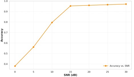
The sensitivity analysis of the GADF-CNN model evaluates its performance under different Signal-to-Noise Ratio (SNR) levels. Gaussian noise is added to the input data based on the specified SNR, and the model’s accuracy is calculated for each SNR level. The results show that the model's accuracy improves as the SNR increases, demonstrating its sensitivity to noise (Fig. 7). At an SNR of 30 dB, the model achieves an accuracy of 0.9708, indicating its robustness to high-quality signals.

In summary, evaluating statistical indicators is crucial for assessing the GADF-CNN approach’s performance and reliability in defect detection. Uncertainty quantification, confidence interval estimation, and sensitivity analysis provide insights into the model’s confidence, accuracy range, and robustness to noise. These indicators collectively offer a comprehensive understanding of the model’s performance, limitations, and potential issues, enabling informed decision-making for real-world applications. The results demonstrate the model’s high consistency, reliability, and accuracy, particularly in high-quality signal scenarios.

4.3. Comparative evaluation of defect recognition models

In this study, a comprehensive comparative analysis was conducted to evaluate five distinct models designed for detecting defects in concrete structures. These models encompass the established architectures of vgg16, resnet18, densenet, resnext50, and the newly developed GADF-CNN model. To ensure equitable comparison, all conventional models – vgg16, resnet18, densenet, and resnext50 – were initialized with pre-trained parameters, utilizing transfer learning from the dataset in question. The training and testing of all models were performed on the NVIDIA Tesla T4 GPU. The results of the defect detection models are illustrated in Fig. 8 and 9.

The initial model evaluated was vgg16, which recorded a training duration of 112.37 seconds and achieved a test accuracy of 92.40 %. Despite its high accuracy, vgg16 exhibited the longest training time among the models evaluated. Subsequently, the resnet18 model underwent training and testing, requiring 31.43 seconds. While faster in training compared to vgg16, it also demonstrated a notable increase in test accuracy to 97.66 %. The densenet and resnext50_32x4d models were next in the sequence of evaluation. The densenet model required 84.45 seconds for training and attained a test accuracy of 95.91 %. In comparison, the resnext50_32x4d model took a marginally longer training time of 110.66 seconds, achieving an identical test accuracy of 95.91 %. Lastly, the newly developed GADF-CNN model was assessed. Its training time was 30.75 seconds, slightly quicker than resnet18 and significantly faster than the other models. Notably, the GADF-CNN model surpassed all other models in test accuracy, reaching 98.24 %.

Fig. 8Training time of vgg16, resnet18, densenet, resnext50, and GADF-CNN

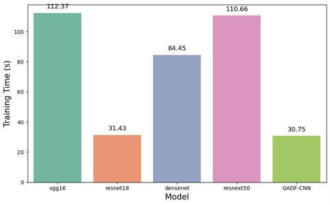
Fig. 9Recognition accuracy of vgg16, resnet18, densenet, resnext50, and GADF-CNN

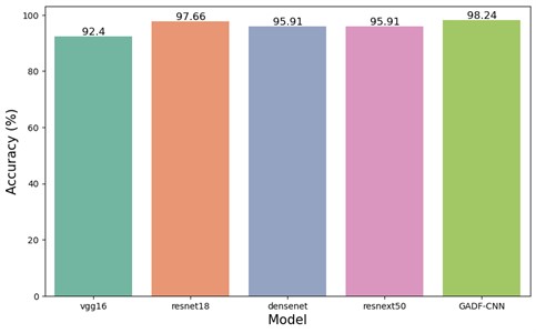
The results indicate that the GADF-CNN model surpasses other models in terms of accuracy and achieves this enhanced performance within a shorter training duration. Consequently, GADF-CNN demonstrates a commendable synergy between computational efficiency and predictive accuracy, establishing its potential as an effective and efficient tool for detecting defects in concrete structures. These findings bolster the assertion that the amalgamation of GADF with a CNN-based depth network, enhanced by Depthwise Separable Convolutions and Attention Mechanisms, leads to a more advanced, precise, and efficient approach for non-destructive testing and evaluation of concrete structures.

To provide additional context for the performance of the GADF-CNN model, a comparative analysis was conducted against a range of methods documented in existing literature. Table 5 presents a summary of the performance metrics of these methods applied to various datasets. The table includes a comparative evaluation of different defect recognition methods for concrete structures, assessed using accuracy, recall, precision, and F1-score metrics. The methods evaluated encompass the Naive Bayes classifier, Support Vector Machines (SVM), standard Convolutional Neural Networks, 1D Convolutional Neural Networks, and the GADF-CNN.

Analysis of Table 5 reveals that the Naive Bayes classifier, as investigated by Jafari et al. [10], demonstrates robust performance with an overall score of 0.92. However, its foundational assumption of feature independence may limit its applicability to more intricate datasets. The SVM application by Dorafshan et al. [13] yields an accuracy of 0.88, but the absence of additional metrics precludes a comprehensive assessment. SVM’s effectiveness is notably dependent on kernel selection and may be less suitable for large, multi-class datasets. Convolutional Neural Network approaches, as reported in studies [14] and [16], achieve accuracies of 0.94 and 0.96, respectively, illustrating the potential of deep learning in this field. However, the lack of complete metric evaluation hinders a full appraisal of these models. The 1D Convolutional Neural Network implemented by Xu et al. [18] exhibits consistent results across metrics, achieving 0.91, which highlights the efficacy of CNNs in processing 1D data. The GADF-CNN model, in contrast, surpasses these with an accuracy of 0.98 and high recall, precision, and F1-score metrics (0.97, 0.97, and 0.98, respectively). This model adeptly merges GADF image transformation with CNN, enhancing defect detection in impact-echo data.

The incorporation of the GADF alongside CNN represents a notable advancement in the realm of non-destructive testing and measurement science at large. By merging sophisticated image transformation techniques with the capabilities of deep learning, this method has demonstrated exceptional efficacy in identifying defects within concrete structures, evidenced by its exemplary performance across accuracy, precision, recall, and F1 score metrics. These outcomes not only highlight the synergy between mathematical methodologies and machine learning in elevating the precision and reliability of engineering measurements but also suggest a promising direction for future research in this interdisciplinary field.

Moreover, the implications of the GADF-CNN technique extend considerably beyond the realm of detecting concrete imperfections. Its validated efficacy establishes a foundation for the adoption of analogous approaches within diverse sectors of measurement science and technology, especially for the intricate data analysis required in the upkeep of essential infrastructure elements like bridges, tunnels, and pavements. Such broad applicability signals the method’s potential to fundamentally transform the methodologies employed in the critical inspection and maintenance of infrastructure. In addition, the model's computational efficiency, achieved through the use of depthwise separable convolutions, is in line with the ongoing objective to devise analytical tools that are both less resource-intensive and highly effective, particularly pertinent for extensive or real-time monitoring endeavors. This strategy not only propels the field of measurement science forward by facilitating quicker and more scalable monitoring solutions but also underscores the significance of sensitivity analysis in ascertaining the robustness and dependability of these measurement systems. Consequently, while the GADF-CNN model has established a new benchmark in concrete defect detection, its contribution to the evolution of measurement tools is profound, fostering the development of safer, more enduring, and resilient infrastructural frameworks.