Abstract
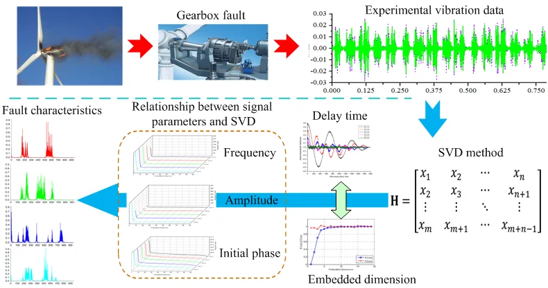
The detection of mechanical fault signals by singular value decomposition is a commonly used method in fault diagnosis. The delay time of the fault signal time series and the rationality of the value of the phase space embedding dimension, as well as the fluctuation of the characteristic parameters of the fault signal, will cause the singular value decomposition method to have a greater impact on the accuracy of fault feature identification and diagnosis. In this article, the simulation model of the similarity signal is established by the combination of the autocorrelation function method and the Cao’s algorithm. Then, the delay time of the signal sequence and the optimal value of the embedded dimension are obtained through simulation. Next, using this method to study the fluctuation of the characteristic parameters such as the frequency, amplitude and initial phase of the signal, the relationship between the characteristic parameters of the signal and the singular value of the signal is obtained. Finally, through the experimental study of the pitting corrosion of the gear tooth surface, the vibration of the fault feature is obtained. The research shows that the combination of autocorrelation function method and Cao's algorithm can calculate the optimal characteristic parameters for the singular value decomposition method and improve the ability of the method to identify fault features.
1. Introduction
In practical applications, mechanical equipment often suffers from various types of failures due to various factors. When the machine equipment fails, it will increase energy consumption and reduce production efficiency. In addition, various types of casualties will be caused by machine failure [1]. Moreover, the formation and development of early faults of the machine is difficult to predict in advance. When the fault causes significant vibration and generates a lot of noise, the state of the fault feature has developed to a more serious level [2]. Therefore, online monitoring of the healthy operation of mechanical equipment is one of the hotspots of current research. Because the on-site environment incorporates the influence of various subjective factors, it causes serious interference to the mechanical equipment fault characteristic signal and makes the extraction of fault features more difficult [3]. So, before the fault feature is extracted, it is necessary to perform noise reduction processing on the fault signal.
In practical applications, there are many methods for signal noise reduction, such as Empirical mode decomposition (EMD) [4, 5], Local mean decomposition (LMD) [6, 7], Singular value decomposition (SVD) [8-10], And wavelet de-noising analysis [11-13] and other methods. Among these noise reduction methods, the reliability and wideness of their applications are limited because some methods have certain defects and their application effects are not good. However, the singular value decomposition method has a good nonlinear filtering effect, and it has been widely used in the fields of noise reduction processing and fault feature recognition of rotating machinery fault signals. For example, Cai J. et al., using the singular value decomposition method to analyze the actual bearing fault data, shows that the method can effectively identify the typical faults of rolling bearings and improve the diagnostic effect of rolling bearing faults [14, 15]. In the application of gear fault diagnosis, the singular value decomposition method is proposed to study the fault type of gears by using the feature extraction method of singular value decomposition. The experimental results show that the method can accurately diagnose and identify different fault types of gears under variable working conditions [16, 17].
The singular value decomposition method is based on the singular value matrix of the characteristic signal, and distinguishes the singular value of the effective feature from the singular value of the noise feature. It is discarding the characteristic information of the noise signal and reconstructing the useful feature signal. The method can be applied to the filtering of nonlinear signals, and has good invariance and stability, which can effectively reduce the noise in the signal [18]. Moreover, in the application of gear fault characteristic signal de-noising and fault identification, it is also proved that the singular value decomposition method (SVD) has strong practical value. In addition, the method can also compress the scale of the fault feature matrix, reduce the difficulty of calculation, and save the consumption of computing resources. However, this method has strong sensitivity to the values of time delay of signal sequence and embedding dimension of phase space in terms of signal noise reduction and accuracy of fault identification. The method of calculating these parameters has no reliable theoretical support and is highly subjective. In response to this problem, scholars generally use the -SVD method [19, 20] to calculate or optimize the time delay and embedding dimension of the signal sequence, so that the accuracy of noise reduction or fault feature recognition can reach a high level. In addition, the singular value decomposition method noise reduction effect and fault feature recognition accuracy are affected by the characteristic parameters of the own algorithm, and are also affected by the characteristic parameters of the external signal, such as the frequency, amplitude and initial phase of the signal. It is still rare to study the influence of signal parameter fluctuation on the singular value decomposition and noise reduction, as well as the variation law between them.
On this basis, based on the advantages of singular value decomposition de-noising method and the principle of noise reduction, the signal's autocorrelation function method and the Cao's algorithm are used to calculate the optimal delay time and embedding dimension of the characteristic signal parameter value. Then, the characteristic signal containing noise is subjected to singular value decomposition to obtain a singular value matrix of the signal. In addition, based on the information characteristics of the fault signal, the autocorrelation function simulation model of the similarity signal is established, and then the simulation method is used to calculate the autocorrelation of the signal sequence over the entire delay time scale, and the optimal delay of each type of signal can be obtained. Next, the Cao's algorithm is used to study the distribution of the signal in the high embedding dimension phase space, obtaining the value of the optimal embedding dimension of the similarity signal. Finally, the effectiveness and practical significance of singular value decomposition, combined with autocorrelation function and Cao’s algorithm for fault feature diagnosis are verified by the experiment of gear tooth surface pitting fault.
2. Theoretical background
2.1. The basic principle of singular value decomposition
The noise reduction method using singular value decomposition is separable for the vibration energy of the effective signal and the noise signal. For a matrix containing noise signals, first separate it according to the principle of singular value decomposition. Then, the singular value of the effective signal is preserved, and the singular values of the noise signal are all set to 0. Finally reconstructed according to the appropriate order, and then the process of obtaining the effective signal after noise reduction.
According to the above research, the singular value decomposition method has a good effect in the field of fault characteristic signal de-noising and fault identification. In mathematical theory, singular value decomposition [21, 22] (SVD) is a method of orthogonalization calculation of a real matrix . No matter whether the row and column of the matrix are related, there are two matrices and matrices such that Eq. (1) holds [23]:
where singular value matrix is a real matrix , , is the singular value of the real matrix , and make , .
Set a set of discrete random time domain signals , its signal sequence can be represented by . By using the singular value decomposition method, the noise in the signal can be filtered out. The operation process is as follows:
1) According to the characteristics of the random signal , a real matrix, namely Hankel matrix is constructed:
where, is dimension of the matrix .
2) Singular value decomposition of matrices according to Eq. (2). Orthogonal matrix , is the singular value matrix of the matrix .
3) Since the Hankel matrix is full rank matrix, the elements , ,⋅⋅⋅, of the singular value matrix are sorted. Satisfy the condition: .
4) Find the mutation point of the singular value in step (3), reserved point previous singular value , and set all the singular values after the point to 0, such as .
5) According to formula , the difference spectrum of singular values in step (4) is calculated, and the order corresponding to the maximum value is found from the difference spectrum of singular values. Then, the singular value is reconstructed according to the order , that is, the signal obtained after the reconstruction is the characteristic signal after noise reduction.
2.2. Determine the time delay of the signal sequence
In the process of signal reconstruction, the selection of the delay time parameter is very critical. When the value of is small, it will cause a serious correlation between the elements in the delay time series. It also leads to no difference between the elements, and the trajectory of the phase space is compressed to the main diagonal, so that the noise dominates the phase space of the reconstructed characteristic signal [24, 25]. When value is large, the correlation between elements in the phase space of the reconstructed feature signal is reduced, resulting in serious loss of reconstruction information. Therefore, when reconstructing the effective feature signal, a reasonable delay time value must be selected to ensure the validity of the reconstructed signal.
Suppose a measured time series is , and the autocorrelation function of the sequence after normalization is shown in Eq. (3):
where is the length of the sample; is the delay time; is the average value of the sample, .
The research shows that the autocorrelation function is used to select the delay time to make the autocorrelation function value exactly attenuate to the time corresponding to , which is the optimal value of the effective phase space eigenvector delay time.
2.3. Determine the embedding dimension of the signal sequence
The Cao’s algorithm, which is the Improved False Nearest Neighbors (IFNN) method, it is used to calculate the embedding dimension of the characteristic signal. The calculation principle as follows [26, 27]:
1) Assume that in an dimension ‘Embedding Space’, the vector time series at the phase point is shown in Eq. (4):
where is the signal corresponding to the time series; is the time series number, ; is the delay time. Calculate the Euclidean distance from the sequence to the nearest neighbor , as shown in Eq. (5):
where is the -norm of the signal sequence.
2) When the dimensional phase space is extended to the 1 dimension, the same vector sequence at the phase point is . Calculate the Euclidean distance from the sequence to the nearest neighbor , as in Eq. (6):
3) Note that means the th reconstructed vector with embedding dimension from Eq. (4). Similar to the idea of the false neighbor method, and we define . From the definition of , one can see that the threshold value should be determined by the derivative of the underlying signal, therefore, for different phase points , should have different threshold values at least in principle. Furthermore, different time series data may have different threshold values. These imply that it is very difficult and even impossible to give an appropriate and reasonable threshold value which is independent of the dimension and each trajectory’s point, as well as the considered time series data. To avoid the above problem, we instead define the relationship between and , as shown in Eqs. (7) and (8):
4) Continue to increase the dimension of the phase space, and make , and repeat the calculation of the first three steps. According to the result of each calculation, draw a diagram of the relationship between and . When a value in the graph tends to be stable within certain threshold, the corresponding to the value is the optimal embedding dimension of the feature signal.
5) However, in the finite sequence of practical applications, it is difficult to discriminate whether the change in value is stable as increases. Therefore, it is necessary to add a criterion, as shown in Eqs. (9) and (10):
Studies have shown that for a random time series, the value of is always equal to 1; For a deterministic time series, the value of is not equal to 1 within a certain threshold.
3. Simulation analysis
3.1. Relationship between SVD and signal frequency
According to the above analysis of the singular value of the analog signal, it is found that there is a certain correlation between the signal frequency and the singular value. In this section, the coupled signals formed by different frequency segment signals and combined in different ways are simulated and calculated to study the variation law between signal frequency and singular value.
3.1.1. Sampling summation of signal frequencies
The simulated signal of the sampled signal frequency is composed of two sets of sinusoidal signals of different frequencies and a random noise signal , shown in Eq. (11). There are five groups of frequency , and some simulation parameters are set to, 1, 0; The simulation parameters of the random white noise signal : the mean is 0, and the variance is 0.7:
1) Relationship between autocorrelation function and delay time.
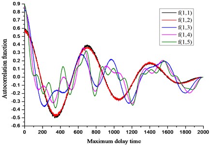
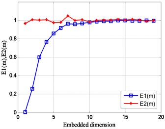
According to the calculation principle of the autocorrelation function method, the five sets of similarity signals of Eq. (11) are respectively subjected to autocorrelation simulation calculation, and the results shown in Fig. 1 are obtained. From the relationship between the autocorrelation function of each signal and the maximum delay time in the figure, it is concluded that the more the number of frequencies including the sub-signal in the analog signal, the attenuation of the white noise signal is more significant with the delay time delay. In addition, the delay time values of the five sets of analog signals are large from the figure.
Fig. 1Relationship between autocorrelation function and delay time
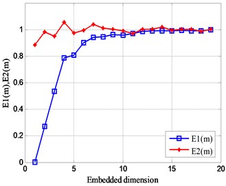
2) Relationship between and embedded dimension .
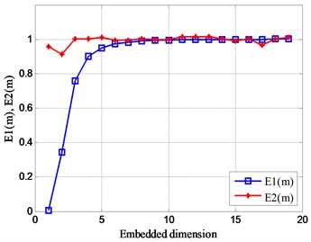
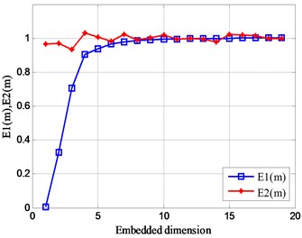
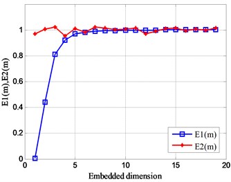
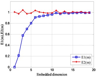
According to the analysis results of Fig. 1, the modified Cao’s algorithm is used to simulate the relationship between the values of the five sets of analog signals and the embedded dimension , and the results are shown in Fig. 2. It can be seen from the figure that when the number of sub-signals containing different frequencies in the analog signal is increasing, the frequency of fluctuates up and down in 1, and the embedding dimension corresponding to the wobble region also becomes larger. The values of are not always 1, indicating that these five sets of analog signals have a certain and unique mode of motion. In addition, the number of sub-signals of different frequencies superimposed on the analog signal has little effect on the value of . Therefore, the optimal embedding dimension of the five sets of analog signals is roughly reasonable between 10 and 15.
Fig. 2Relationship between Em and embedded dimension m
a)
b)
c)

d)
e)
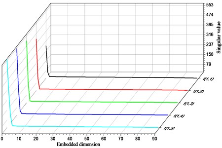
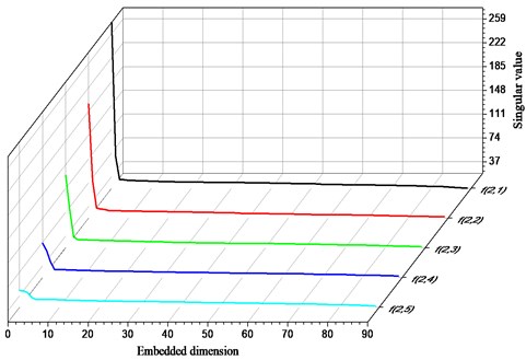
The singular value of the analog signal increases as the number of frequency signals superimposed in the signal increases, and it is also proportional to the frequency value in Fig. 3. In addition, the fluctuation of the number of frequencies or the magnitude of the frequency has a great influence on the singular value of the effective characteristic signal, and has no influence on the phase space of the noise signal.
Fig. 3The singular values of different frequency signals
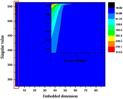
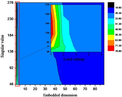
In order to more clearly reflect the difference of the singular values of each signal, the cloud diagram shown in Fig. 4 is used to illustrate the distribution of singular values in its space. As the number of sub-signal products in the analog signal increases, the distribution of the largest singular values is concentrated on the left most top of the graph. The trend of the distribution gradient from the upper right to the lower left gradually decreases, and the width of each gradient gradually increases from large to small. In addition, in the distribution space of the entire singular value, the singular value of 99 % or more is below 54.88.
Fig. 4Distribution of singular value space of analog signal
3.1.2. Sample product of signal frequency
This simulation signal contains the product of a plurality of sinusoidal signals of different frequencies, and a certain amount of random noise signals are combined to form an analog signal . The expression of the analog signal is shown in Eq. (12): This frequency is five groups, the other parameters are the same as above:
Fig. 5Relationship between autocorrelation function and delay time
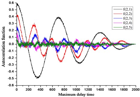
Fig. 6Relationship between Em and embedded dimension m

a)
b)
c)
d)
e)
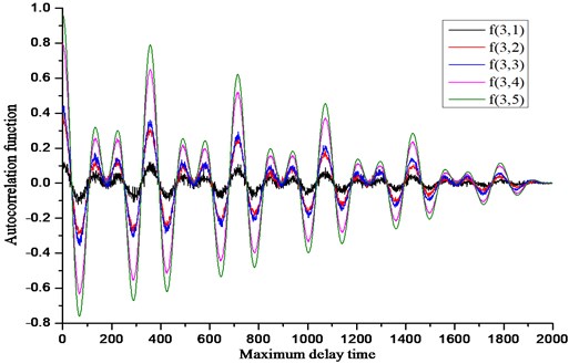
1) Relationship between autocorrelation function and delay time.
In the same way, the analog signal composed of the products of different frequency sub-signals is used in the same way, and the relationship between the analog signal and the delay time is calculated by the autocorrelation function method, and the result is shown in Fig. 5. From this figure, the more the number of sub-signals of different frequencies in the analog signal, the lower the autocorrelation of the signal. In addition, the number of products of different frequency sub-signals has little effect on the attenuation amplitude of the noise signal over the entire delay time scale.
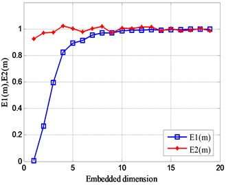
2) Relationship between and embedded dimension .
In the same way, the Cao’s algorithm is used to calculate embedded dimension the analog signals of Eq. (16) respectively, and the calculation results are obtained in Fig. 6.
As the number of sub-signals constituting the analog signal increases, the value of fluctuates slightly above and below 1, and the fluctuation trend of the value of remains stable on the scale of the embedding dimension . At the same time, it is explained that each analog signal has a certain motion characteristic. In addition, the value of is basically 1 in the dimension with the embedding dimension of 10-15, which also shows that the optimal embedding dimension of this set of analog signals can be more reasonable in the dimension value of 10-15.
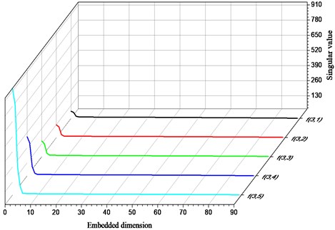
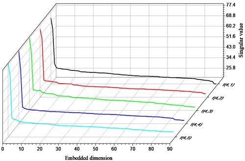
The sampling product of a plurality of frequency signals, the singular value of the analog signal decreases as the number of frequencies increases is shown in Fig. 7. The fluctuation of the number of frequencies or the frequency value has a great influence on the singular value of the effective signal, and the influence on the noise signal is small.
Fig. 7The singular values of different frequency signals
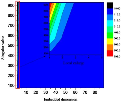
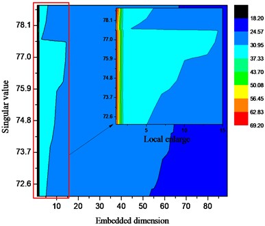
The larger value group of the singular value of the analog signal is mainly concentrated before the embedding dimension is 5 in Fig. 8, and each gradient stripe line approximate to the vertical line is sequentially expanded to the right side. In addition, the singular value is 26.3-33.8, which accounts for about half of the entire singular value space. Therefore, when the feature signal is composed of a plurality of sets of sub-signals of different frequencies, the more the number of sub-signals, the more severe the interference of the effective characteristic information.
3.2. Relationship between SVD and signal amplitude
In this section, the influence of the change of signal amplitude on the singular value of the signal is studied by using the method of simulation. The simulation signal consists of a sinusoidal signal and a random white noise signal . The expression of this signal is shown in Eq. (13). The parameter is set to: the values of the amplitude are , the values of the frequency are , the values of the initial phase are , other parameters are the same as above:
Fig. 8Distribution of singular value space of analog signal
1) Relationship between autocorrelation function and delay time.
In the same way, the variation law between the autocorrelation function and the delay time of each signal is studied by changing the amplitude of the signal, and the result shown in Fig. 9 is obtained. As the amplitude of the analog signal increases, the autocorrelation of each signal increases. At the same time, the autocorrelation of the signal has a high degree of regularity over the entire delay time scale. In addition, as the amplitude of the signal increases, the noise signal is gradually masked.
Fig. 9Relationship between autocorrelation function and delay time
2) Relationship between and embedded dimension .
In the same way, the results of Fig. 10 are obtained through simulation calculation. As the number of signal amplitudes increases, the values of and are basically unchanged. However, as the magnitude of the signal amplitude increases, the value of varies greatly. In addition, the value range of the signal optimal embedding dimension is concentrated between 5 and 10.
Fig. 10Relationship between Em and embedded dimension m
a)
b)
c)
d)
e)
Fig. 11Relationship between amplitude and singular values
The singular value of the analog signal increases as the amplitude increases is shown in Fig. 11. As the amplitude increases, the transition point of the singular value of the analog signal shifts back slightly. In addition, the change of amplitude has the greatest influence on the singular value of the effective signal, and the influence on the noise is weak.
Similarly, the signal amplitude increases monotonically in the forward direction, the value of the useful singular value also increases in the same direction in Fig. 12. However, singular values that may be useful in the entire singular value space account for only about 2 %.
Fig. 12Distribution of singular value space of analog signal
3.3. Relationship between SVD and initial phase of signal
In this section, the simulation analysis method is used to study the relationship between signal phase and signal singular value. The simulation signal consists of an initial sinusoidal signal and a random white noise signal , and the mathematical expression of the simulated signal is shown in Eq. (14). Parameter setting: The values of the frequency are ; the values of the initial phase are , and the other parameters are the same as above:
1) Relationship between autocorrelation function and delay time.
This part is studied the influence of the initial phase on the phase space of the signal by changing the initial phase of the analog signal. According to the set parameters, the results shown in Fig. 13 are obtained through simulation calculation. from this graph, the initial phase also affects the autocorrelation of the signal to a small extent. During a certain delay period, the autocorrelation of the signal increases significantly with the increase of the initial phase. However, on the entire delay time scale, the initial phase of the signal has no effect on the noise attenuation amplitude.
2) Relationship between and embedded dimension .
Similarly, by calculating the change of the initial phase value of the signal, the result shown in Fig. 14 is obtained. It can be obtained from the modification that the initial phase of the signal changes, and the value of fluctuates slightly between 1 and 5, and its value always 1 after the dimension 5. Explain that the initial state of the signal changes without affecting the distribution of the signal phase space. In addition, the value of is always 1 after the dimension 5. This shows that the optimal embedding dimension of this set of analog signals is 5.
Fig. 13Relationship between autocorrelation function and delay time
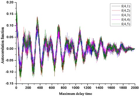
Fig. 14Relationship between Em and embedded dimension m
a)
b)
c)
d)
e)
The singular value of the analog signal is substantially unchanged as the initial phase increases in Fig. 15. However, the change in the initial phase has a significant effect on the noise signal.
Fig. 15Relationship between initial phase and singular value
The fluctuation of the initial phase value of the analog signal has less influence on the magnitude of the useful singular value is shown in Fig. 16. However, the distribution that can lead to useful singular values becomes more complicated. In addition, the fluctuation of the initial phase mainly affects the characteristic information of singular values within 24.57-30.95. At the same time, the singular value of this kind of feature accounts for about 80 %, and the gradient of its distribution is more complicated. This shows that when the state of the initial phase of the signal changes, it does not cause interference to the main feature information, but it affects the characteristic state of the noise signal.
Fig. 16Distribution of singular value space of analog signal
4. Experimental verification
4.1. Experimental setup
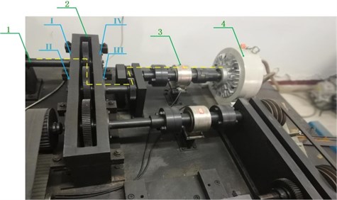
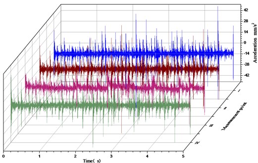
In this section, the fixed-axis gear unit structure and the tooth surface pitting failure of the gear teeth are tested to verify the effectiveness of the singular value decomposition de-noising method. In the gearbox under test, spur gears were used as the research object for this experiment. The layout of the test bench is shown in Fig. 17. On the outside of the gearbox bearing support, four test points are set: measuring point I, measuring point II, measuring point III and measuring point IV. Four similar uniaxial acceleration sensors are installed at the four measuring points to collect the acceleration value of the fault vibration.
The input speed is 1500 r/min; the input current of the magnetic powder loader is 0.1 A; the experimental object is the spur gear, the modulus 22 mm, the number of teeth 55, and the tooth width 20 mm. The material of the gear is 18CrNiMo7 steel.
Fig. 17Structural layout of the test bed: 1 – motor input shaft; 2 – measured gear box; 3 – torque transducer; 4 – magnetic powder loader
4.2. Analysis of experimental results
1) Experimental data.
The time domain values of the vibration acceleration at the four measuring points were collected by experiment, as shown in Fig. 18. It can be seen from the figure that the experimental data at the four measuring points are affected by a large number of interference signals, so the vibration characteristics at the test position are not obvious, and the noise reduction processing of the measured experimental data is required.
Fig. 18Time domain diagram of vibration acceleration at points before noise reduction
2) Calculate the delay time.
According to the calculation principle of the autocorrelation function method, the delay time of the time series of the fault vibration signals at the four measuring points is calculated separately, and the calculation results is shown in Table 1.
Table 1The delay time of signals at each points
Measuring point | I | II | III | IV |
Delay time | 2 | 2 | 2 | 2 |
3) Calculate the embedded dimension.
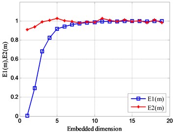
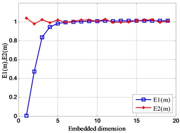
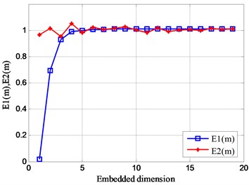
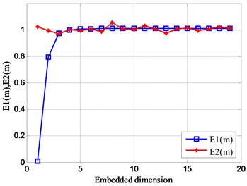
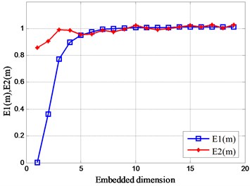
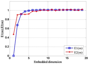
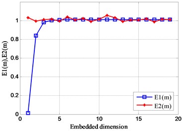
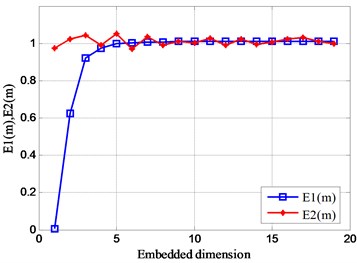
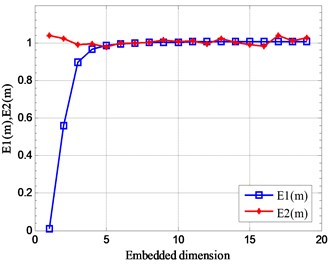
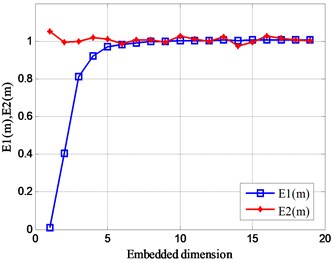
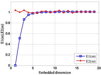
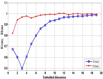
According to the improved Cao’s algorithm, the optimal embedding dimension of the vibration signal at the four test positions on the gearbox is calculated separately in Fig. 19. It can be seen from the figure that the value of is not equal to 1, indicating that the four measuring points have certain vibration characteristics. In addition, is close to a constant value of 1 for the first time when the embedding dimension is equal to 19. Therefore, the optimal embedding dimension of the vibration signal at these four measuring points is equal to 19.
Fig. 19Relationship between Em and m of experimental signals
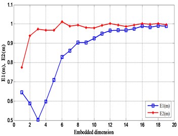
a) Measuring point I
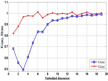
b) Measuring point II
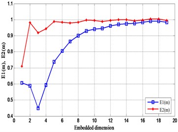
c) Measuring point III
d) Measuring point IV
4) Singular value decomposition of experimental data.
According to the singular value decomposition theory, combined with the simulation principle of singular value decomposition method. In this section, use the same analysis method to perform singular value decomposition on the experimental data at the measuring point I, the measuring point II, the measuring point III and the measuring point IV. The singular value decomposition parameter is set to: hysteresis time 2, initial order 90. After the singular value decomposition, the calculation result is shown in Fig. 20. The singular values of the four measuring points all have abrupt changes at the position of 1000 in Fig. 20(a). Theoretically, the value is the boundary point between the effective signal and the noise signal, but the singular value after the point is still high. In addition, the singular value is gradually reduced gradually, but the singular value energy is still high; and the singular value difference spectrum is obtained before the 5th order in Fig. 20(b), and the spectrum value is the largest. At the same time, the difference spectrum values at positions of 10, 20, 64, etc. are approximately 100. It is indicated that the part after the singular value of 1000 also contains a certain amount of valid information.
5) Analysis of fault vibration characteristics.
The experimental data after the noise reduction is subjected to Fourier calculation, and the frequency response diagram at each measurement point is obtained in Fig. 21. The measuring points II and III are coaxial with the input power source, and the vibration of the power source is greatly affected. The vibration at the position of the measuring point is complicated. The measuring points I and IV are coaxial with the load.
Fig. 20Singular values of fault signals at each points
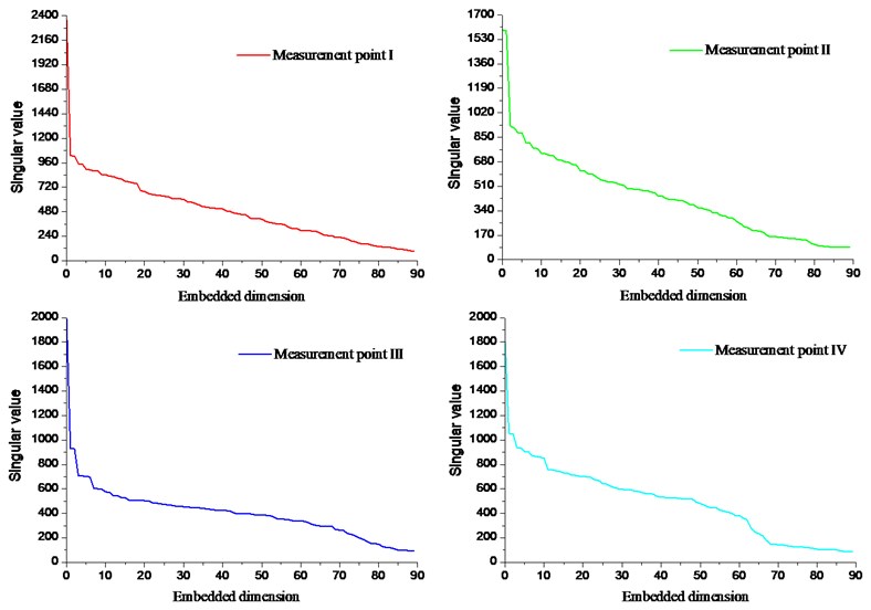
Fig. 21Frequency of fault signals at each point
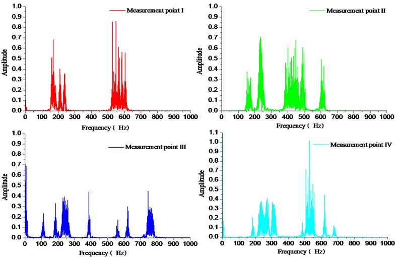
However, the measuring point I is far away from the load and less affected by the load vibration. Therefore, the vibration characteristics of the measuring point I are only related to the fault vibration characteristics, and the low frequency vibration amplitude is large. The measuring point IV close to the load, and the vibration characteristics at the measuring point are affected by the load excitation. In addition, it is possible to derive the fault vibration at the four measuring points on the gearbox, and a large-cycle frequency doubling resonance phenomenon is generated with the transmission system.
5. Conclusions
This article first expounds the basic principles of noise reduction and fault identification for singular value decomposition. Secondly, the accuracy of the noise reduction and fault feature recognition of the singular value decomposition method is analyzed, which is mainly affected by the delay time of the signal sequence and the value of the phase space embedding dimension. Finally, the influence of the fluctuation of singular value and signal characteristic parameters on the fault characteristics is studied by means of simulation. Through the research of this paper, the following conclusions are drawn:
1) According to the characteristics of the fault signal sequence, the simulation model of various analog signals is established by the autocorrelation function method. After the simulation calculation, the value of the optimal delay time of each analog signal is obtained. The relationship between the autocorrelation of the signal and the maximum delay time is studied, and the attenuation of the fault characteristics and noise information over the entire time scale is obtained.
2) According to the calculation principle of the improved Cao’s algorithm, the optimal embedding dimension values of each analog signal are calculated.
3) Using the autocorrelation function method of the signal and the improved Cao's algorithm, the relationship between the fluctuation degree of the characteristic parameters such as the frequency, amplitude and initial phase of the external signal and the singular value of the signal is studied.
4) Through the fault test of the gear, it is verified that the method has high effectiveness and reliability for the noise reduction effect and fault feature recognition of the gear fault characteristic signal.
References
-
Lu C., Wang Z., Qin W., et al. Fault diagnosis of rotary machinery components using a stacked denoising autoencoder-based health state identification. Signal Processing, Vol. 130, 2017, p. 377-388.
-
Qiao Z., Lei Y., Li N. Applications of stochastic resonance to machinery fault detection: A review and tutorial. Mechanical Systems and Signal Processing, Vol. 122, 2019, p. 502-536.
-
Asr M. Y., Ettefagh M. M., Hassannejad R., et al. Diagnosis of combined faults in rotary machinery by non-naive Bayesian approach. Mechanical Systems and Signal Processing, Vol. 85, 2017, p. 56-70.
-
Huang N., Shen Z., Long S., et al. The empirical mode decomposition and the Hilbert spectrum for non-linear and nonstationary time series analysis. Proceedings of the Royal Society of London, Vol. 454, 1998, p. 903-995.
-
Tong S., Zhang Y., Xu J., et al. Pattern recognition of rolling bearing fault under multiple conditions based on ensemble empirical mode decomposition and singular value decomposition. Journal of Mechanical Engineering Science, Vol. 232, 2017, p. 2280-2296.
-
Smith J. S. The local mean decomposition and its application to EEG perception data. Journal of the Royal Society Interface, Vol. 2, 2005, p. 443-454.
-
Philipp Z., Daniel F. P., Stephan R. Active control of planetary gearbox vibration using phase-exact and narrowband simultaneous equations adaptation without explicitly identified secondary path models. Mechanical Systems and Signal Processing, Vol. 120, 2019, p. 234-251.
-
Lei R., Shang P. New irreversibility measure and complexity analysis based on singular value decomposition. Physica A: Statistical Mechanics and its Applications, Vol. 212, 2018, p. 913-924.
-
Bie F., Horoshenkov K. V., Qian J., et al. An approach for the impact feature extraction method based on improved modal decomposition and singular value analysis. Journal of Vibration and Control, Vol. 25, Issue 5, 2019, p. 1096-1108.
-
Cheng L., Chen L., Liang T., et al. Features of singular value decomposition and its application to the vibration monitoring of turboprop engine. Communication, Signal Processing, and Systems, Vol. 463, 2019, p. 1495-1506.
-
Shu X., Han S. Improvement of DOA estimation using wavelet denoising. 1st International Conference on Information Science and Engineering, 2009, p. 587-590.
-
Abdeldjalil O. A review of wavelet denoising in medical imaging. 8th International Workshop on Systems, Signal Processing and their Applications (WoSSPA), 2013, p. 19-26.
-
Golestani A., Kolbadi S. S. M., Ali A. Localization and de-noising seismic signals on SASW measurement by wavelet transform. Journal of Applied Geophysics, Vol. 98, 2013, p. 124-133.
-
Li H., Zhang Q., Qin X., et al. K-SVD based WVD enhancement algorithm for planetary gearbox fault diagnosis under a CNN framework. Measurement Science and Technology, 2019. doi:10.1088/1361-6501/ab4488.
-
Cai J., Xiao Y. Bearing fault diagnosis method based on the generalized S transform time-frequency spectrum de-noised by singular value decomposition. Proceedings of the Institution of Mechanical Engineers, Part C: Journal of Mechanical Engineering Science, Vol. 233, Issue 7, 2019, p. 2467-2477.
-
Xing Z., Qu J., Chai Y., et al. Gear fault diagnosis under variable conditions with intrinsic time-scale decomposition-singular value decomposition and support vector machine. Journal of Mechanical Science and Technology, Vol. 31, Issue 2, 2017, p. 545-553.
-
Qin Y., Zhang Q., Zhao Y. Fault diagnosis method for planetary gearboxes based on adaptive SVD. Zhendong yu Chongji/Journal of Vibration and Shock, Vol. 37, Issue 17, 2018, p. 122-127.
-
Li L., Cui Y., Chen R., et al. Optimal SES selection based on SVD and its application to incipient bearing fault diagnosis. Shock and Vibration, Vol. 2018, 2018, p. 8067416.
-
Yang H., Lin H., Ding K. Sliding window denoising K-Singular Value Decomposition and its application on rolling bearing impact fault diagnosis. Journal of Sound and Vibration, Vol. 421, 2018, p. 205-219.
-
Tang N., Tong S., Xu J., et al. Research on feature extraction based on short-time series reconstruction and K-SVD. Machine Design and Research, Vol. 34, Issue 4, 2018, p. 18-22.
-
Zeng M., Yang Y., Zheng J., et al. μ-SVD based denoising method and its application to gear fault diagnosis. Journal of Mechanical Engineering, Vol. 51, Issue 3, 2015, p. 95-103.
-
Juan M., Tomas S. SVD update methods for large matrices and applications. Linear Algebra and its Applications, Vol. 561, 2019, p. 41-62.
-
Merainani B., Rahmoune C., Benazzouz D., et al. A novel gearbox fault feature extraction and classification using Hilbert empirical wavelet transform, singular value decomposition, and SOM neural network. Journal of Vibration and Control, Vol. 24, 2017, p. 2512-2531.
-
Li H., Liu T., Wu X., et al. Research on bearing fault feature extraction based on singular value decomposition and optimized frequency band entropy. Mechanical Systems and Signal Processing, Vol. 118, 2019, p. 477-502.
-
Ma J., Wu J., Wang X. A hybrid fault diagnosis method based on singular value difference spectrum denoising and local mean decomposition for rolling bearing. Journal of Low Frequency Noise, Vibration and Active Control, Vol. 37, 2018, p. 928-954.
-
Luo Y. Comparative study on traffic flow prediction based on ESN and Elman neural networks. Journal of Hunan University of Technology, Vol. 27, 2013, p. 67-72.
-
Cao L., Wu S., Zhao H. Chaos in topological Markov chains. Systems Science and Mathematical Sciences, Vol. 7, 1994, p. 97-105.
About this article

This work is supported by the National Natural Science Foundations of China (No. 51175419) and Shaanxi Key Laboratory of Machinery Manufacturing Equipment Construction Project, which are highly appreciated by the authors.
Xintao Zhou contributions in this paper are writing papers, providing research methods, investigation, validation, and experimental verification, etc. Yahui Cui contributions in this paper are formal analysis, funding acquisition, and investigation, etc. Na Ma contributions are assisting thesis writing, thesis translation and experiments, etc. Xiayi Liu contribution is to provide simulation schemes, and paper translation, etc. Longlong Li contributions are the typesetting of papers, and revision of the English language, etc. Lihua Wang contribution was the review and editing of paper.
