Research on singular spectrum decomposition and its application to rotor failure detection

Pang, Bin; Tang, Guiji; He, Yuling

doi:10.21595/jve.2018.19200

Journal of Vibroengineering

Browse Journal

Submit article

Published: 30 September 2018

Check for updates

Research on singular spectrum decomposition and its application to rotor failure detection

Bin Pang¹

Guiji Tang²

Yuling He³

^{1, 2, 3}School of Energy, Power and Mechanical Engineering, North China Electric Power University, Baoding, 071003, China

Corresponding Author:

Guiji Tang

Cite the article Download PDF

Downloads 1742

WoS Core Citations 1

CrossRef Citations 2

Abstract

As an important part of rotating machinery, a healthy rotor is critical to ensuring optimal working conditions of the entire system. Considering that the vibration signal of rotor consists of different frequency components when the failure arises, a novel rotor failure detection method based on singular spectrum decomposition (SSD) is presented. The original vibration signal is adaptively decomposed into a number of singular spectrum components (SSCs) by the SSD method. Then, energy separation algorithm (ESA) is adopted to demodulate each singular spectrum component. Finally, the SSD-ESA time-frequency spectrum can be obtained and the fault features contained in the SSD-ESA time-frequency spectrum can be identified to determine the fault types. The effectiveness of SSD for harmonic separation was assessed through tones separation analyses, the results show that SSD is able to separate more harmonic pairs of different amplitude ratios than empirical mode decomposition (EMD). Furthermore, three simulations of multi-component signals were designed to investigate the use of SSD for signal decomposition. The SSD method was then applied to detect signatures caused by rotor oil film whirl in experimental signals and compared to both EMD and ensemble EMD (EEMD). The simulated analysis results reflect that SSD shows superiority to EMD and EEMD in inhibiting mode mixing and extracting the time-varying frequency components. The experimental analysis results demonstrate that the SSD based rotor failure detection method is an alternative method under both constant and variable speed conditions.

Research on singular spectrum decomposition and its application to rotor failure detection

Highlights

Singular spectrum decomposition (SSD) is used to decompose the vibration signal of the defective rotors.
A SSD-ESA time-frequency method is proposed with the combination of SSD and energy separation algorithm (ESA).
The SSD-ESA time-frequency can extract the fault features of rotors more accurately compared to the EMD-HT and EEMD-HT time-frequency methods.
The proposed method can diagnose rotor faults under both constant and variable speed conditions.

1. Introduction

As a main transmission and bearing mechanism of rotating machinery, the rotor plays a pivotal role in the industrial production [1]. With the improvement of the production efficiency, the rotating machinery is growing faster, enduring heavier load, becoming more automated and more complicated, which increases the failure rates of rotors. Rotor condition monitoring and failure detection are of significance to ensure the production safety and avoid the economic loss [2].

The existing research results show the fault vibration signal of rotor contains abundant information of fault features. Therefore, rotor fault diagnosis methods based on vibration analysis have attracted focused attention and are widely applied in practice [3]. The vibration signals of common rotor failures, such as oil whirl, oil film oscillation, rubbing, and cracks, are composed of the harmonic components that are related to the rotor rotating frequency. In order to separate the harmonic signals successfully, varieties of signal decomposition methods have been applied in rotor failure detection, such as empirical mode decomposition (EMD) [4], ensemble EMD (EEMD) [5], local mean decomposition (LMD) [6], ensemble LMD (ELMD) [7, 8], intrinsic time-scale decomposition (ITD) [9], local characteristic-scale decomposition (LCD) [10], complete overall LCD (CELCD) [11], differential-based EMD (DEMD) [12], differential-based EEMD (DEEMD) [13], etc. While these signal decomposition methods have solved some rotor fault diagnosis problems effectively in the applications, envelope fitting must be performed during the decomposition process to successfully obtain the intrinsic mode functions (IMFs) [14]. Consequently, the problem of mode mixing always exists and the decomposition results can be easily affected by abnormal noise and interferences [15]. In recent years, some other parametric-based signal decomposition methods such as the morphological component analysis (MCA) [16, 17], empirical wavelet transform (EWT) [18-20], synchro squeezed wavelet transform (SWT) [21, 22], adaptive local iterative filtering (ALIF) [23, 24], and variational mode decomposition (VMD) [25, 26] have also been put forward to improve the decomposition effects for multi-component signals and applied to rotor fault diagnosis successfully. However, the problem of parameter selection needs to be solved in order to get a good result and it increases the complexity of fault diagnosis. Moreover, during actual operating processes rotors frequently operate under variable speed conditions and traditional signal decomposition methods lose their effectiveness when analyzing time-varying non-stationary signals.

Considering the above problems, a recently developed signal decomposition method, namely singular spectrum decomposition (SSD) is introduced into rotor fault diagnosis in this work. The SSD algorithm is highly based on singular spectrum Analysis (SSA) [27], which has been proved suitable for analyzing non-stationary time series. The advantages of SSD are that it cannot only set the amount of embedding dimension but also select the principal components to choose for reconstructing a specific component series adaptively. Therefore, SSD is a nonparametric decomposition technique and has qualified precision. The time-frequency spectrum consists of the instantaneous frequency (IF) and instantaneous amplitude (IA) of each component of the rotor vibration signal can reflect the health status of the rotor [28]. Combining the signal decomposition methods with the demodulation techniques to perform the time-frequency analysis has been frequently used for rotor failure detection. In this paper, SSD is utilized to separate the rotor failure vibration signal into several singular spectrum components (SSCs). Then, demodulation analysis as a further process is required to calculate the IF and IA of each SSC. Hilbert transform (HT) [29] and energy separation algorithm (ESA) based on Teager-Kaiser energy operator (TKEO) [30] are two of the most well-known demodulation techniques. HT is a linear integral operator while TKEO is a nonlinear operator which is based on differentiation [31]. The ESA demodulation method based on TKEO can compute the IF and IA without involving integral transforms as in HT. ESA has a promising demodulation performance and low computational complexity [32]. Here, ESA is combined with SSD to get the SSD-ESA time-frequency spectrum in order to provide the judgments for rotor fault diagnosis.

The subsequent contents are organized as follows. Section 2 outlines the principles of the SSD based failure detection technique. In Section 3, the SSD method is assessed via tone separation analysis. In Section 4, simulated analyses are performed to evaluate SSD. In Section 5, experimental verifications are conducted. Lastly, conclusions are drawn in Section 6.

2. The proposed method for rotor fault diagnosis

2.1. Singular spectrum decomposition

SSD is a newly proposed and creative signal decomposition technique which is originated from SSA. Despite SSA has shown the effectiveness in analyzing and predicting non-stationary time series in the previous studies, previous studies suggest a number of challenges exist in automatically setting the value of the embedding dimension and selecting the principal components to reconstruct a signal component that has physical meanings. An improvement of SSD relative to SSA is that it can choose the SSA fundamental parameters adaptively. The decomposed components, referred to as SSCs, can be iteratively derived. The specific implementation steps of every iteration are as follows.

1) Constructing the trajectory matrix.

Given an input signal $y (n)$ with the length of $N$ , if the embedding dimension is set to $M$ , an ( $M \times N$ ) matrix $Y$ will be constructed and its $i$ th row would be achieved as:

y_{i} = [y (i), \dots, y (N), y (1), \dots, y (i - 1)] .

Hence, $Y = {[y_{1}^{T}, y_{2}^{T}, \dots, y_{M}^{T}]}^{T}$ . For a given series, $y (n) = \{1,2, 3,4, 5\}$ , if $M$ is set to 3, the trajectory matrix $Y$ comes to be:

1

Y = [\begin{array}{l} 1 & 2 & 3 & 4 & 5 \\ 2 & 3 & 4 & 5 & 1 \\ 3 & 4 & 5 & 1 & 2 \end{array}] .

The selection of the embedding dimension $M$ has an important impact on the analysis results. For SSD, $M$ is adaptively chosen as $f_{m a x} / f_{s}$ , $f_{m a x}$ is the dominant frequency in the power spectral density (PSD) of $y (n)$ , $f_{s}$ represents the sampling frequency.

A modified matrix $X$ is obtained by adjusting the positions of some elements of $Y$ shown as follows:

2

X = [\begin{array}{l} 0 & 0 & 1 & 0 & 0 \\ 0 & 1 & 2 & 0 & 0 \\ 1 & 2 & 3 & 4 & 5 \\ 2 & 3 & 4 & 5 & 0 \\ 3 & 4 & 5 & 0 & 0 \end{array}] .

The original can be extracted with the application of the diagonal averaging to the modified matrix. This transform will also be adopted in step (3) to extract a singular spectrum component.

2) Decomposition.

The singular value decomposition is performed on the trajectory matrix $Y$ , defined as:

3

Y = U D V^{T} = [u_{1}, u_{2}, \dots, u_{M}] [\begin{matrix} λ_{1} & 0 & 0 & 0 & 0 \\ 0 & λ_{2} & \dots & 0 & 0 \\ ⋮ & ⋮ & ⋱ & ⋮ & 0 \\ 0 & 0 & \dots & λ_{M} & 0 \end{matrix}] [\begin{matrix} {v_{1}}^{T} \\ {v_{2}}^{T} \\ ⋮ \\ {v_{N}}^{T} \end{matrix}] = λ_{1} u_{1} {v_{1}}^{T} + λ_{2} u_{2} {v_{2}}^{T}

+ \dots + λ_{M} u_{M} {v_{M}}^{T} = H_{1} + H_{2} + \dots + H_{M},

where, $U \in R^{M \times M}$ and $V \in R^{N \times N}$ , include the left and right singular vectors, individually. Both belong to orthogonal matrices. $D \in R^{M \times N}$ is the singular values matrix.

3) Grouping and reconstruction.

As shown in Eq. (3), the trajectory matrix $Y$ can be expressed as the sum of $M$ principle components. The $L$ ( $L < M$ ) principle components, whose left eigenvectors exhibits a domain frequency in the frequency range [ $f_{m a x} - Δ f$ , $f_{m a x} + Δ f$ ], are selected to reconstruct a wanted singular spectrum component. $Δ f$ is estimated through a Gaussian interpolation of the PSD of the input signal.

Assume that the selected $L$ principle components contribute to a new matrix $Z$ . We can get the corresponding estimated component by conducting the diagonal average on the modified matrix obtained from the transform of $Z$ as described in Eq. (2).

The estimated singular spectrum component is then subtracted from $y (n)$ . The above process is performed on the residual iteratively until a stopping criterion is met.

More details about SSD can be found in [27].

2.2. The ESA demodulation based on TKEO

TKEO is an energy tracking method which is originally developed for speech processing [33], for which a continuous signal $s (t)$ is defined as:

4

Ψ [s (t)] = [\dot{s} (t)]^{2} - s (t) \ddot{s} (t),

where $\dot{s} (t)$ and $\ddot{s} (t)$ represent the first and second derivatives of $s (t)$ . The corresponding discrete expression of the TKEO is given:

5

Ψ [s (n)] = [s (n)]^{2} - s (n + 1) s (n - 1) .

From Eq. (5), only three samples are needed for computing the instant energy. Therefore, TKEO possesses a positive time resolution and is easy to carry out expeditiously. The ESA demodulation based on TKEO was previously developed to estimate the IF and IA of a mono-component amplitude and frequency modulated (AM-FM) signal [34], as follows:

6

f (t) = \frac{1}{2 π} \sqrt{\frac{Ψ [\dot{s} (t)]}{Ψ [s (t)]}},

7

|A (t)| = \frac{Ψ [s (t)]}{\sqrt{Ψ [\dot{s} (t)]}} .

From this, a number of discrete energy separation algorithms have been developed, including the discrete ESA-1(DESA-1) [34] that will be used here and is given by:

8

f (n) = a r c c o s (1 - \frac{Ψ [y (n)] + Ψ [y (n + 1)]}{4 Ψ [s (n)]}),

9

A (n) = \sqrt{\frac{ψ [s (n)]}{1 - {(1 - \frac{Ψ [y (n)] + Ψ [y (n + 1)]}{4 Ψ [y (n)]})}^{2}}},

where $y (n) = s (n) - s (n - 1)$ represents the backward asymmetric difference of $s (n)$ .

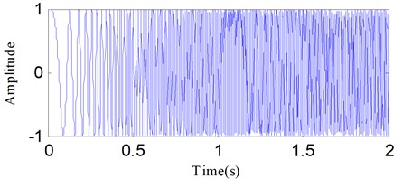
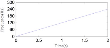
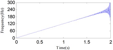
A linear frequency modulation signal $x (t)$ shown in the following equation is simulated to evaluate the demodulation performance of DESA-1. The sampling frequency is 1024 Hz:

10

x (t) = c o s (2 π 60 t^{2}) .

The time waveform of $x (t)$ is shown in Fig. 1. Both DESA-1 and HT are employed to calculate the IA and IF of the linear frequency modulation signal. Fig. 2 and 3 show the estimated results of IA and IF using the two methods. The results demonstrate that the demodulation performance of DESA-1 is a little better. Both the IF and IA estimated by HT exhibit a worse end effects problem. The cause for the end effect in HT demodulation is associated with a circular convolution issue [35].

Fig. 1The simulated linear frequency modulation signal

ESA is a good demodulation method, but only fit for analyzing the mono-component signals. Then, a filter bank method must be performed on the original signal to obtain the mono-components firstly. For this work, SSD is used as the filter bank method.

Fig. 2The instantaneous amplitudes of the linear frequency modulation signal calculated using DESA-1 and HT: a) DESA-1, b) HT

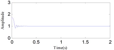
a)

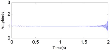
b)

Fig. 3The instantaneous frequencies of the linear frequency modulation signal calculated using DESA-1 and HT: a) DESA-1, b) HT

a)

b)

2.3. The SSD-ESA time-frequency analysis

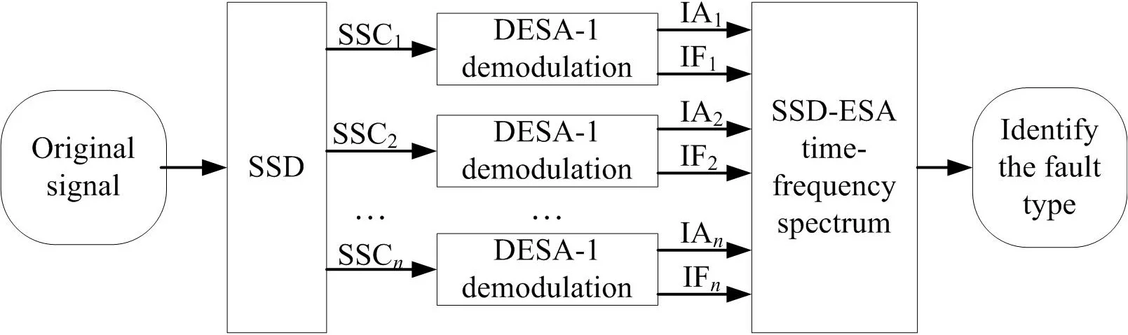
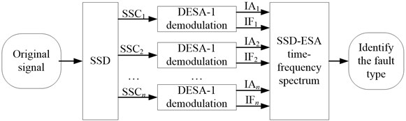
Based on the merits of SSD and ESA, a time frequency method called SSD-ESA is proposed for rotor failure detection. A flowchart of the SSD-ESA method is shown in Fig. 4. The method can be implemented by followings steps:

1) Decompose the rotor vibration signal into some monocomponents ( $n$ SSCs) using SSD.

2) Calculate the IF and IA of each SSC using the DESA-1 demodulation.

3) Obtain the SSD-ESA time-frequency spectrum by combing all the demodulation results of monocomponents.

4) Identify the fault type according to the SSD-ESA time-frequency spectrum.

Fig. 4The flow chart of the SSD-ESA time-frequency analysis

3. Tones separation analysis

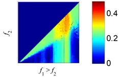
A massive challenge for the signal decomposition methods is the separation of two different superimposed tones [36]. The following input signal adopted in [36] is used to evaluate the effectiveness of SSD for tones separation:

11

y_{f_{1}, f_{2}} (t) = a_{1} c o s 2 π f_{1} t + a_{2} c o s 2 π f_{2} t,

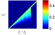
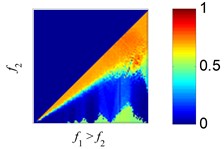
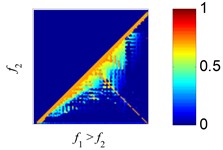
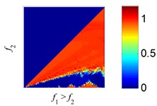
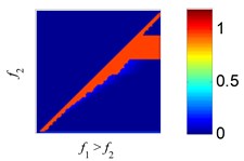
with $f_{2} < f_{1} < f_{s}$ , $a_{1}$ and $a_{2}$ are the amplitudes of the two pure harmonics. Here, we define a function to represent the amplitude ratio, $r = a_{1} / a_{2}$ Both EMD and SSD are applied to decompose the superimposed tones with varying amplitude ratios $r \in \{4, 1, 1 / 4\}$ , and the estimated errors in the extraction are calculated with the same way in [36]. The results are displayed in Fig. 5.

As the results reflect, EMD exhibits large, different regions of confusion, where the two harmonics with close frequency can’t be separated correctly, as reported in [36]. Using SSD, the regions with large estimated errors decrease relative to EMD, indicating SSD can separate more tone pairs than EMD. As the results show, SSD exhibits high decomposition accuracy across most of the domain, except where $f_{1}$ and $f_{2}$ are approximately equal.

Fig. 5The estimation errors of EMD and SSD in the process of 2 tones separation: a), c) and e) are the estimation error plots of EMD, b), d) and f) are the estimation error plots of SSD. The amplitude ratios are set to r= 4, 1, 1/4

The estimation errors of EMD and SSD in the process of 2 tones separation: a), c) and e) are the estimation error plots of EMD, b), d) and f) are the estimation error plots of SSD. The amplitude ratios are set to r= 4, 1, 1/4

a) EMD, $r =$ 4

b) SSD, $r =$ 4

c) EMD, $r =$ 1

d) SSD, $r =$ 1

e) EMD, $r =$ 1/4

f) SSD, $r =$ 1/4

4. Simulation analysis

Rotor vibration signals are always influenced by abnormal events, including noise and other types of interferences, these abnormal events can cause the problem of mode mixing in traditional signal decomposition methods such as EMD, EEMD. Another problem is that existing methods for rotor fault diagnosis are difficult to deal with the variable speed conditions. Therefore, SSD is investigated on three different multi-component signals to validate its effectiveness for signal decomposition. Simulations are performed in MATLAB (R2012a) using a desktop computer with a 3.30 GHz Pentium Dual-Core CPU and 4.0 GB of RAM.

4.1. Simulation 1

In order to show the SSD robustness with respect to noise, the signal $x_{1} (t)$ is given for testing, which is composed of three components, i.e., an AM–FM signal $x_{11} (t)$ , an amplitude modulated signal $x_{12} (t)$ , and a random noise signal $x_{13} (t)$ . The expression of $x_{1} (t)$ is presented as:

12

\{\begin{array}{l} x_{1} (t) = x_{11} (t) + x_{12} (t) + x_{13} (t), \\ x_{11} (t) = 2 s i n (4 π t) s i n [200 π t + s i n (10 π t)], \\ x_{12} (t) = c o s (4 π t) s i n (100 π t), \\ x_{13} (t) = 0.6 r a n d (1, N), \end{array}

where, $N =$ 1024, is the signal length. The sampling frequency $f_{s} =$ 1024 Hz.

Fig. 6 shows the three components of $x_{1} (t)$ . First, SSD is applied to decompose $x_{1} (t)$ . Fig. 7 shows the decomposed results. We can find that SSC₁ and SSC₃ are respectively corresponding to $x_{11} (t)$ and $x_{12} (t)$ . For comparison, EMD and EEMD are used to decompose $x_{1} (t)$ and the first four decomposed IMFs are shown in Figs. 8 and 9, respectively. The IMFs obtained by using EMD and EEMD exhibit mode mixing in addition to false components, and both methods fail to obtain the original components of $x_{1} (t)$ . SSD has a stronger ability to resist the noise than EMD and EEMD.

Fig. 6The components of x1t

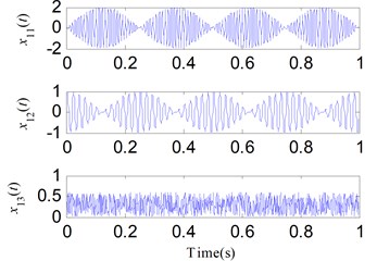
Fig. 7The decomposed results of x1t using SSD

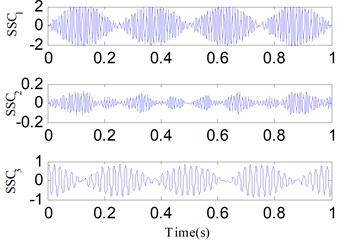
Fig. 8The first four decomposed IMFs of x1t using EMD

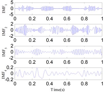
Fig. 9The first four decomposed IMFs of x1t using EEMD

Three kinds of evaluating indexes including the root mean squared error (RMSE) [37, 38], correlation coefficient (CC) [39] and consuming time for the whole decomposition process [38] are employed to evaluate the decomposition performances of the SSD, EMD and EEMD methods. The smaller RMSE and the greater CC values represent the decomposition results are more accurate. Taking the SSD method as an example, from [38], the RMSE is defined as:

13

R M S E = \sqrt{E [(m (t) - S S C (t))^{2}]},

where $m (t)$ and $S S C (t)$ respectively denote the real component and the corresponding SSC obtained by SSD. The definition of the correlation coefficient is as follows [39]:

14

C C = \frac{C O V (m (t), S S C (t))}{\sqrt{V a r (m (t))} \sqrt{V a r (S S C (t))}},

where $C O V (m (t)$ , $S S C (t))$ is the covariance of $m (t)$ and $S S C (t)$ , $V a r (m (t))$ and $V a r (S S C (t))$ respectively represent the variance of $m (t)$ and $S S C (t)$ .

The decomposed components of SSC₁ and SSC₃ obtained by SSD, IMF₁ and IMF₃ obtained by EMD, IMF₁ and IMF₃ obtained by EEMD are selected to compute the RMSE and CC indexes with the corresponding true components of $x_{1} (t)$ . To evaluate the calculation efficiency, the total time required for each decomposition method was calculated using the “tic-toc” function in MATLAB. Results are shown in Table 1. The RMSE values of the SSD method are clearly smaller than for the EMD and EEMD methods, and the CC values of the SSD method are higher. The EMD method takes the least time to accomplish the decomposition and the consuming time of the SSD method is less than the EEMD method. The evaluation results suggest that the SSD method is the most accurate and has satisfactory efficiency.

Table 1The evaluating indexes for the SSD, EMD and EEMD methods used in simulation 1

Methods	RMSE		Correlation coefficient		Consuming time (s)
Methods	$x_{11} (t)$	$x_{12} (t)$	$x_{11} (t)$	$x_{12} (t)$	Consuming time (s)
SSD	0.1120	0.0946	0.9950	0.9933	0.097530
EMD	0.5498	0.3329	0.8391	0.7587	0.044772
EEMD	0.4237	0.3118	0.9059	0.7935	8.183337

4.2. Simulation 2

The second simulated signal $x_{2} (t)$ is formed by a cosine signal $x_{21} (t)$ , a linear frequency modulation signal $x_{22} (t)$ and an interval signal $x_{23} (t)$ as the following equation:

15

\{\begin{array}{l} x_{2} (t) = x_{21} (t) + x_{22} (t) + x_{23} (t), \\ x_{21} (t) = c o s (100 π t), \\ x_{22} (t) = 0.6 c o s (10 π t + 10 π t^{2}), \\ x_{23} (t) = \{\begin{array}{l} \begin{matrix} 0.3 c o s (200 π t), & \begin{matrix} 0.2 < t < 0.25, 0.4 < t < 0.45, \\ 0.6 < t < 0.65, 0.8 < t < 0.85, \end{matrix} \end{matrix} \\ 0, o t h e r w i s e, \end{array} \end{array}

where, $N =$ 1024, is the number of sampling points of $x_{2} (t)$ . The sampling frequency $f_{s} =$ 1024 Hz.

The three components of $x_{2} (t)$ are given in Fig. 10. SSD, EMD and EEMD are used to separate the mixed signal $x_{2} (t)$ for comparisons. Figs. 11-13 show the corresponding separation results respectively. As shown in the results, the SSD method decompose $x_{2} (t)$ into three SSCs, and $S S C_{1}$ , $S S C_{2}$ , $S S C_{3}$ are respectively corresponding to $x_{23} (t)$ , $x_{21} (t)$ and $x_{22} (t)$ . EMD and EEMD are failed to separate the components of $x_{2} (t)$ . The analysis results indicate that the interference can cause mode mixing when using EMD and EEMD, while SSD has a better performance in anti-interference.

The evaluating indexes, RMSE, CC, and consuming time, were compared for Simulation 2, and are presented in Table 2. The SSD method has the highest precision according to the RMSE and CC values. Moreover, SSD is more efficient than EEMD.

4.3. Simulation 3

To validate the effectiveness of SSD in extracting the time-varying frequency components, we design the third simulated signal $x_{3} (t)$ , which comprises two linear frequency modulation signals, namely $x_{31} (t)$ , $x_{32} (t)$ , and a random noise signal $x_{33} (t)$ . The former two represent the time--varying frequency components. Eq. (16) is the specific expression of $x_{3} (t)$ :

16

\{\begin{array}{l} x_{3} (t) = x_{31} (t) + x_{32} (t) + x_{33} (t), \\ x_{31} (t) = c o s [2 π (20 + 40 t) t], \\ x_{32} (t) = 0.5 c o s [6 π (20 + 40 t) t], \\ x_{33} (t) = 0.15 r a n d (1, N), \end{array}

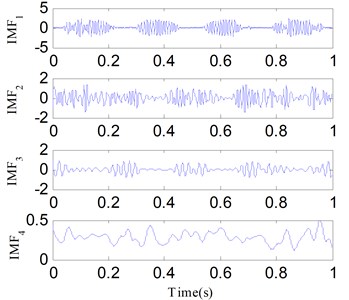
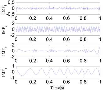
where, the sampling number $N$ is 512 and the frequency sampling frequency $f_{s}$ is 1024 Hz. Fig. 14 illustrates the components of $x_{3} (t)$ . For comparison, $x_{3} (t)$ is analyzed by SSD, EMD and EEMD simultaneously. Figs. 15-17 show their analysis results respectively. SSC₁ represents the noise component, while SSC₂ and SSC₃ respectively correspond to the components $x_{31} (t)$ and $x_{32} (t)$ . The IMF₂ and IMF3 of EMD and EEMD are similar to $x_{31} (t)$ and $x_{32} (t)$ , but they endure serious mode mixing and waveform distortion problems. The results suggest the SSD method is effective in separating time-varying frequency components, making it a suitable alternative method for rotor failure detection under variable speed conditions.

Table 2The evaluating indexes for the SSD, EMD and EEMD methods used in simulation 2

Methods	RMSE			Correlation coefficient			Consuming time (s)
Methods	$x_{21} (t)$	$x_{22} (t)$	$x_{23} (t)$	$x_{21} (t)$	$x_{22} (t)$	$x_{23} (t)$	Consuming time (s)
SSD	0.0075	0.0129	0.0186	0.9999	0.9996	0.9804	0.182506
EMD	0.3714	0.2909	0.3029	0.8530	0.7291	0.0027	0.103784
EEMD	0.1919	0.2346	0.2996	0.9671	0.8376	0.0063	8.229770

Fig. 10The components of x2t

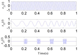
Fig. 11The decomposed results of x2t using SSD

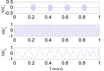
Fig. 12The first four decomposed IMFs of x2t using EMD

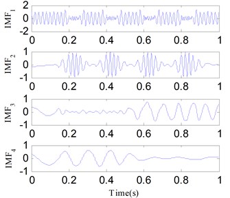
Fig. 13The first four decomposed IMFs of x2t using EEMD

Again, a comparison is conducted based on the three evaluating indicators and the results are reflected in Table 3. The contrasting results suggest that the SSD method offers the best decomposition performance and decreases the consuming time compared with EEMD.

Table 3The evaluating indexes for the SSD, EMD and EEMD methods used in simulation 3

Methods	RMSE		Correlation coefficient		Consuming time (s)
Methods	$x_{31} (t)$	$x_{32} (t)$	$x_{31} (t)$	$x_{32} (t)$	Consuming time (s)
SSD	0.0540	0.0730	0.9973	0.9792	0.167045
EMD	0.3647	01958	0.8648	0.8409	0.035285
EEMD	0.3055	0.1475	0.9034	0.9094	7.238292

5. Experimental analysis

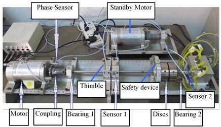
The Bently RK-4 test rig, shown in Fig. 18, was used to simulate an oil film whirl fault under either constant or variable speed conditions. The power source of the test bench comes from an electric motor and the motor drives the system directly through a flexible coupling.

The main components of the rig include a motor, a speed-adjusting controller, two sliding bearings, two discs, and one oil feeding system. A phase sensor is installed near the coupling to monitor the rotating speed and a safety device is designed to ensure a safe contact experiment. Oil film whirl signals are derived from eddy current sensor 1 and sensor 2 by monitoring the shaft vibration. The sampling frequency $f_{s} =$ 1280 Hz.

Fig. 14The components of x3t

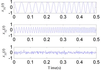
Fig. 15The decomposed results of x3t using SSD

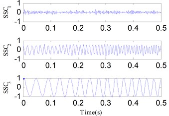
Fig. 16The first four decomposed IMFs of x3t using EMD

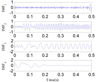
Fig. 17The first four decomposed IMFs of x3t using EEMD

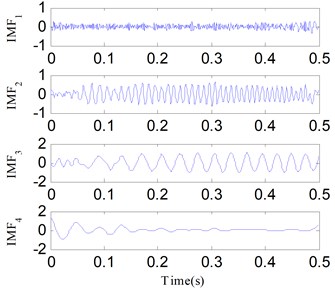
Fig. 18Rotor system test rig

5.1. Oil film whirl fault diagnosis under constant speed condition

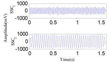
The first critical speed of the test rig is about 1900 r/min. Experiment results show the oil film whirl fault arises when the rotation speed is about 1600-1700 r/min after several tests in this test rig. The oil film whirl will evolve into oil film whip when the rotation speed is about 3700-3800 r/min. The previous studies denote that the vibration signal oil film whirl fault mainly contains two frequency components, $f_{r}$ (representing the rotating frequency) and about 1/2 $f_{r}$ . So, the oil film whirl is also called half frequency whirl. The oil film whirl fault under a constant rotating frequency, i.e., $f_{r} =$ 46.7 Hz, is performed and Fig. 19 shows the time waveform. An analysis for the signal in Fig. 19 is conducted with the proposed method. Fig. 20(a) exhibits the decomposition components obtained by SSD, two SSCs are obtained. Both the DESA-1 and HT method are used to demodulate the two SSCs. As a result, the SSD-ESA and the SSD-HT time-frequency spectrums are obtained as reflected in Fig. 20(b) and Fig. 20(c) separately. Both the SSD-ESA and SSD-HT time-frequency spectrums suggest that the instantaneous frequencies of the two SSCs are $f_{r}$ and 1/2 $f_{r}$ respectively corresponding to the fault features of an oil film whirl fault.

Fig. 19The oil film whirl signal under constant speed condition

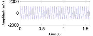
Fig. 20The analysis results of the signal in Fig. 19 using the SSD method: a) the decomposed SSCs via SSD, b) the SSD-ESA time-frequency spectrum, c) the SSD-HT time-frequency spectrum

The analysis results of the signal in Fig. 19 using the SSD method: a) the decomposed SSCs via SSD, b) the SSD-ESA time-frequency spectrum, c) the SSD-HT time-frequency spectrum

a)

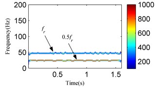
b)

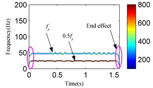
c)

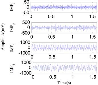
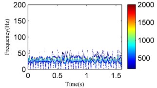
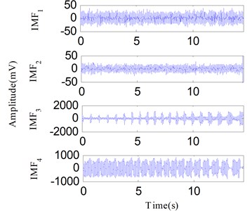
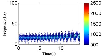
However, the SSD-HT time-frequency spectrum exhibits worse end effects compared to the SSD-ESA time-frequency spectrum. For a further comparison, the EMD-HT and EEMD-HT time-frequency analyses are performed on the oil film whirl vibration signal. The results are respectively given in Figs. 21 and 22. The IMFs obtained by EMD and EEMD reflect serious mode mixing and false components are also observed. Furthermore, the EMD-HT and EEMD-HT time-frequency spectrums failed to extract the accurate fault characteristic frequencies.

5.2. Oil film whirl fault diagnosis under variable speed condition

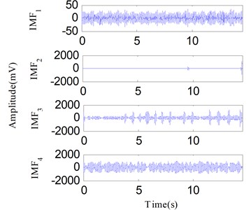
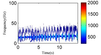
In the actual production process, the rotor must support variable speed conditions. Detecting rotor failures under variable speed conditions is a challenging task. The test bench in Fig. 18 can complete the step-less speed regulation within the scope of 0-10000 r/min by adjusting the speed-adjusting controller. To carry out the experiment for an oil film whirl fault under the variable speed condition, the rotational speed was gradually increased from zero to a maximum speed just under 3800 r/min. The vibration signal was analyzed as the rotational speed was increased to 1800-2400 r/min and the signal waveform is illustrated in Fig. 23. The vibration signal is also decomposed into two components by SSD as Fig. 24(a) shows. Fig. 24(b) and Fig. 24(c) respectively show the SSD-ESA and SSD-HT time-frequency spectrums. The instantaneous frequencies of the SSCs are $f_{r}$ and 1/2 $f_{r}$ for each time-frequency spectrum. It is visible that the time-frequency aggregation of the SSD-ESA method is a little better. Results for the EMD-HT and EEMD-HT methods are shown in Figs. 25 and 26, respectively. It’s a pity that both methods failed to separate the two potential characteristic frequencies. The proposed method shows an advantage in failure detection under variable speed conditions.

Fig. 21The analysis results of the signal in Fig. 19 using the EMD method: a) the first four IMFs obtained by EMD, b) the EMD-HT time-frequency spectrum

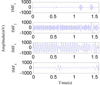
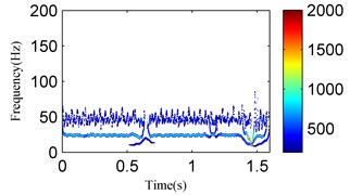
a)

Fig. 22The analysis results of the signal in Fig. 19 using the EEMD method: a) the first four IMFs obtained by EEMD, b) the EEMD-HT time-frequency spectrum

The analysis results of the signal in Fig. 19 using the EEMD method: a) the first four IMFs obtained by EEMD, b) the EEMD-HT time-frequency spectrum

a)

b)

Fig. 23The oil film whirl signal under variable speed condition

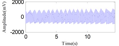
Fig. 24The analysis results of the signal in Fig. 23 using the SSD method: a) the decomposed SSCs using SSD, b) the SSD-ESA time-frequency spectrum, c) the SSD-HT time-frequency spectrum

The analysis results of the signal in Fig. 23 using the SSD method: a) the decomposed SSCs using SSD, b) the SSD-ESA time-frequency spectrum, c) the SSD-HT time-frequency spectrum

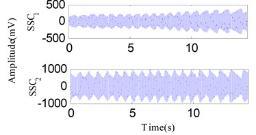
a)

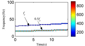
b)

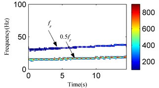
c)

Fig. 25The analysis results of the signal in Fig. 23 using the EMD method: a) the first four IMFs obtained by EMD, b) the EMD-HT time-frequency spectrum

a)

b)

Fig. 26The analysis results of the signal in Fig. 23 using the EEMD method: a) the first four IMFs obtained by EEMD, b) the EEMD-HT time-frequency spectrum

The analysis results of the signal in Fig. 23 using the EEMD method: a) the first four IMFs obtained by EEMD, b) the EEMD-HT time-frequency spectrum

a)

b)

6. Conclusions

In this paper, the SSD method is used to separate the rotor failure vibration signal to get satisfactory decomposition results. Moreover, the SSD-ESA time-frequency spectrum is applied to detect the signatures of rotor failures. Tones separation investigations demonstrate that SSD has a better performance in tones separation compared with EMD. The simulation results suggest SSD is capable of improving the decomposition precision and is superior to both EMD and EEMD in overcoming mode mixing. Two vibration signals representing an oil film whirl fault are experimentally examined under either constant speed or variable speed conditions. The results exhibit that SSD can successfully extract the fault feature components and the potential characteristic information can be identified from the SSD-ESA time-frequency spectrum. In conclusion, the proposed method is superior to traditional methods.

References

Hu A., Hou L., Xiang L. Dynamic simulation and experimental study of an asymmetric double-disk rotor-bearing system with rub-impact and oil-film instability. Nonlinear Dynamics, Vol. 84, Issue 2, 2015, p. 1-19.

Search CrossRef
Peng Z., He Y., Lu Q., et al. Feature extraction of the rub-impact rotor system by means of wavelet analysis. Journal of Sound and Vibration, Vol. 259, Issue 4, 2003, p. 1000-1010.

Publisher
Nembhard A. D., Sinha J. K., Yunusa Kaltungo A. Development of a generic rotating machinery fault diagnosis approach insensitive to machine speed and support type. Journal of Sound and Vibration, Vol. 337, 2015, p. 321-341.

Publisher
Cheng J., Yu D., Tang J., et al. Local rub-impact fault diagnosis of the rotor systems based on EMD. Mechanical Systems and Signal Processing, Vol. 44, Issue 4, 2009, p. 784-791.

Search CrossRef
Lei Y., Li N., Lin J., et al. Fault diagnosis of rotating machinery based on an adaptive ensemble empirical mode decomposition. Sensors, Vol. 13, Issue 12, 2013, p. 16950-16954.

Publisher
Cheng J. S., Yang Y., Yang Y. A rotating machinery fault diagnosis method based on local mean decomposition. Digital Signal Processing, Vol. 22, Issue 2, 2012, p. 356-366.

Publisher
Yang Y., Cheng J. S., Zhang K. An ensemble local mean decomposition and its application to local rub-impact fault diagnosis of the rotor systems. Measurement, Vol. 45, 2012, p. 561-570.

Publisher
Sun J., Xiao Q., Wen J., et al. Natural gas leak location with K-L divergence-based adaptive selection of ensemble local mean decomposition components and high-order ambiguity function. Journal of Sound and Vibration, Vol. 347, 2015, p. 232-245.

Publisher
Frei M. G., Osorio I. Intrinsic time-scale decomposition: time-frequency-energy analysis and real-time filtering of non-stationary signals. Proceedings Mathematical Physical and Engineering Sciences, Vol. 463, 2007, p. 321-342.

Publisher
Cheng J. S., Zheng J. D., Yang Y. A nonstationary signal analysis approach – the local characteristic – scale decomposition method. Journal of Vibration Engineering, Vol. 25, Issue 2, 2012, p. 215-220.

Search CrossRef
Zheng J. D., Cheng J. S., Nie Y. H., et al. Complete ensemble local characteristic-scale decomposition and its applications to rotor fault diagnosis. Journal of Vibration Engineering, Vol. 27, Issue 4, 2014, p. 637-646.

Search CrossRef
Li M., Li F., Jing B., et al. Complete ensemble local characteristic-scale decomposition and its applications to rotor fault diagnosis. Journal of Vibration and Control, Vol. 21, Issue 9, 2015, p. 1821-1837.

Search CrossRef
Li H., et al. Multi-faults decoupling on turbo-expander using differential-based ensemble empirical mode decomposition. Mechanical Systems and Signal Processing, Vol. 93, 2017, p. 267-280.

Publisher
Lei Y., He Z., Zi Y. Application of the EEMD method to rotor fault diagnosis of rotating machinery. Mechanical Systems and Signal Processing, Vol. 23, Issue 4, 2009, p. 1327-1338.

Publisher
Tang B., Dong S., Song T. Method for eliminating mode mixing of empirical mode decomposition based on the revised blind source separation. Signal Processing, Vol. 92, Issue 1, 2012, p. 248-258.

Publisher
Starck J. L., Moudden Y., et al. Morphological component analysis. Proceedings of SPIE, 2005, p. 5194.

Publisher
Chen X., Yu D., Luo J. Early rub-impact diagnosis of rotors using morphological component analysis. Journal of Vibration Engineering, Vol. 27, Issue 3, 2014, p. 466-472.

Search CrossRef
Gilles J. Empirical Wavelet Transform. IEEE Transactions on Signal Processing, Vol. 61, Issue 16, 2013, p. 3999-4010.

Publisher
Li Z., Zhu, M., Chu, F., et al. Mechanical fault diagnosis method based on empirical wavelet transform. Chinese Journal of Scientific Instrument, Vol. 35, Issue 11, 2014, p. 2423-2432.

Search CrossRef
Chen F., Ye Y., Chen W., et al. Fault diagnosis of motorized spindle via modified empirical wavelet transform-kernel pca and optimized support vector machine. Journal of Vibroengineering, Vol. 19, Issue 4, 2017, p. 2611-2631.

Publisher
Daubechies I., Lu J., Wu H. T. Synchrosqueezed wavelet transforms: An empirical mode decomposition-like tool. Applied and Computational Harmonic Analysis, Vol. 30, Issue 2, 2011, p. 243-261.

Publisher
Yang H. Synchrosqueezed wave packet transforms and diffeomorphism based spectral analysis for 1D general mode decompositions. Applied and Computational Harmonic Analysis, Vol. 39, Issue 1, 2015, p. 33-66.

Publisher
Cicone A., Liu J., Zhou H. Adaptive local iterative filtering for signal decomposition and instantaneous frequency analysis. Applied and Computational Harmonic Analysis, Vol. 41, Issue 2, 2016, p. 384-411.

Publisher
An X. Local rub-impact fault diagnosis of a rotor system based on adaptive local iterative filtering. Transactions of the Institute of Measurement and Control, Vol. 39, Issue 5, 2016, p. 748-753.

Publisher
Dragomiretskiy K., Zosso D. Variational Mode Decomposition. IEEE Transactions on Signal Processing, Vol. 62, Issue 3, 2014, p. 531-544.

Publisher
Wang Y., Markert R., Xiang J., et al. Research on variational mode decomposition and its application in detecting rub-impact fault of the rotor system. Mechanical Systems and Signal Processing, Vol. 60, 2015, p. 243-251.

Publisher
Bonizzi P., Karel J. M., Meste O., et al. Singular spectrum decomposition: a new method for time series decomposition. Advances in Adaptive Data Analysis, Vol. 6, Issue 4, 2014, p. 1450011.

Publisher
Zeng M., Yang Y., Zheng J., et al. Normalized complex Teager energy operator demodulation method and its application to fault diagnosis in a rubbing rotor system. Mechanical Systems and Signal Processing, Vol. 50, Issue 51, 2015, p. 380-399.

Publisher
Huang N. E., Shen Z., Long S. R., et al. The empirical mode decomposition and the Hilbert spectrum for nonlinear and non-stationary time series analysis. Proceedings of the Royal Society of London A: Mathematical, Physical and Engineering Sciences, Vol. 454, 1998, p. 903-995.

Publisher
Qin Y. Multicomponent AM-FM demodulation based on energy separation and adaptive filtering. Mechanical Systems and Signal Processing, Vol. 38, Issue 2, 2013, p. 440-459.

Publisher
Li H., Zhang Y., Zheng H. Bearing fault detection and diagnosis based on order tracking and Teager-Huang transform. Journal of Mechanical Science and Technology, Vol. 24, Issue 3, 2010, p. 811-822.

Publisher
Bouchikhi A., Boudraa A. O. Multicomponent AM-FM signals analysis based on EMD-B-splines ESA. Signal Processing, Vol. 92, Issue 9, 2012, p. 2214-2228.

Publisher
Maragos P., Kaiser J. F., Quatieri T. F. On amplitude and frequency demodulation using energy operators. IEEE Transactions on Signal Processing, Vol. 41, Issue 4, 1993, p. 1532-1550.

Publisher
Maragos P., Kaiser J. F., Quatieri T. F. Energy separation in signal modulations with application to speech analysis. IEEE Transactions on Signal Processing, Vol. 41, Issue 10, 1993, p. 3024-3051.

Publisher
Antoniadou I., Manson G., Staszewski W. J., et al. A time-frequency analysis approach for condition monitoring of a wind turbine gearbox under varying load conditions. Mechanical Systems and Signal Processing, Vol. 64, 2015, p. 188-216.

Publisher
Rilling G., Flandrin P., Goncalves P. On empirical mode decomposition and its algorithms. IEEE Eurasip Workshop on Nonlinear Signal and Image Processing, Vol. 3, 2003, p. 8-11.

Search CrossRef
Li Y., Xu M., Lang X., et al. Application of bandwidth EMD and adaptive multi-scale morphology analysis for incipient fault diagnosis of rolling bearings. IEEE Transactions on Industrial Electronics, Vol. 64, Issue 8, 2017, p. 6506-6517.

Publisher
Li Y., Xu M., Wei Y., et al. An improvement EMD method based on the optimized rational Hermite interpolation approach and its application to gear fault diagnosis. Measurement, Vol. 63, 2015, p. 330-345.

Publisher
Zheng J., Cheng J., Yang Y. Generalized empirical mode decomposition and its applications to rolling element bearing fault diagnosis. Mechanical Systems and Signal Processing, Vol. 40, Issue 1, 2013, p. 136-153.

Publisher

Cited by

A New Singular Spectrum Decomposition Method Based on Cao Algorithm and Amplitude Aware Permutation Entropy

Hong Yang | Aohan Zhang | Guohui Li

(2021)

Gearbox Fault Diagnosis Based on Hierarchical Instantaneous Energy Density Dispersion Entropy and Dynamic Time Warping

Guiji Tang | Bin Pang | Yuling He | Tian Tian

(2019)

About this article

Received

26 September 2017

Accepted

13 February 2018

Published

30 September 2018

SUBJECTS

Fault diagnosis based on vibration signal analysis

DOI

https://doi.org/10.21595/jve.2018.19200

Keywords

singular spectrum decomposition

energy separation algorithm

variable speed condition

rotor

failure detection

Acknowledgements

This paper is supported by the National Natural Science Foundation of China (Grant No. 51777074, 51307058), and the Fundamental Research Funds for the Central Universities (Grant No. 2017XS134, 2017MS190).

This is an open access article distributed under the Creative Commons Attribution License, which permits unrestricted use, distribution, and reproduction in any medium, provided the original work is properly cited.

Previous article in issue Previous Next article in issue Next

Research article

2018 06 30

Gear fault feature extraction and classification of singular value decomposition based on Hilbert empirical wavelet transform

Rahmoune Chemseddine, Merainani Boualem, Benazzouz Djamel, Fedala Semchedine

Research article

2018 05 15

A novel classification method combining adaptive local iterative filtering with singular value decomposition for fault diagnosis

Yong Lv, Yi Zhang, Cancan Yi, Han Xiao, Zhang Dang

Research article

2017 12 31

Feature extraction method based on VMD and MFDFA for fault diagnosis of reciprocating compressor valve

Yan Liu, Jindong Wang, Ying Li, Haiyang Zhao, Shuxin Chen

Research article

2017 05 15

An adaptive stochastic resonance method for weak fault characteristic extraction in planetary gearbox

Zhixing Li, Boqiang Shi

B. Pang, G. Tang, and Y. He, “Research on singular spectrum decomposition and its application to rotor failure detection,” Journal of Vibroengineering, Vol. 20, No. 6, pp. 2336–2351, Sep. 2018, https://doi.org/10.21595/jve.2018.19200

Copy Extrica

Copied to clipboard!

TY  - JOUR
DO  - 10.21595/jve.2018.19200
UR  - https://doi.org/10.21595/jve.2018.19200
TI  - Research on singular spectrum decomposition and its application to rotor failure detection
T2  - Journal of Vibroengineering
AU  - Tang, Guiji
AU  - Pang, Bin
AU  - He, Yuling
PY  - 2018
DA  - 2018/09/30
PB  - JVE International Ltd.
SP  - 2336-2351
IS  - 6
VL  - 20
SN  - 1392-8716
SN  - 2538-8460
ER  - 

Copy Ris

Copied to clipboard!

@article{Tang_2018,
	doi = {10.21595/jve.2018.19200},
	url = {https://doi.org/10.21595/jve.2018.19200},
	year = 2018,
	month = {sep},
	publisher = {{JVE} International Ltd.},
	volume = {20},
	number = {6},
	pages = {2336--2351},
	author = {Guiji Tang and Bin Pang and Yuling He},
	title = {Research on singular spectrum decomposition and its application to rotor failure detection},
	journal = {Journal of Vibroengineering}
}

Copy Bibtex

Copied to clipboard!

[1]G. Tang, B. Pang, and Y. He, “Research on singular spectrum decomposition and its application to rotor failure detection,” Journal of Vibroengineering, vol. 20, no. 6, pp. 2336–2351, Sep. 2018, doi: 10.21595/jve.2018.19200.

Copy IEEE

Copied to clipboard!

Tang, Guiji, Bin Pang, and Yuling He. “Research on Singular Spectrum Decomposition and Its Application to Rotor Failure Detection.” Journal of Vibroengineering 20, no. 6 (September 30, 2018): 2336–51. https://doi.org/10.21595/jve.2018.19200.

Copy Chicago

Copied to clipboard!

Research on singular spectrum decomposition and its application to rotor failure detection

Abstract

Highlights

1. Introduction

2. The proposed method for rotor fault diagnosis

2.1. Singular spectrum decomposition

2.2. The ESA demodulation based on TKEO

2.3. The SSD-ESA time-frequency analysis

3. Tones separation analysis

4. Simulation analysis

4.1. Simulation 1

4.2. Simulation 2

4.3. Simulation 3

5. Experimental analysis

5.1. Oil film whirl fault diagnosis under constant speed condition

5.2. Oil film whirl fault diagnosis under variable speed condition

6. Conclusions

References

Cited by

About this article

Related Articles