An intelligent fault diagnosis method of rotating machinery based on deep neural networks and time-frequency analysis

1. Introduction

Fault diagnosis and pattern identification are crucial to the health monitoring of rotating machinery, especially for the high speed machinery and its components, such as bearing, gear and rotor in the aircraft engine. Vibration signals of rotating components always exhibit the non-linear and non-stationary characteristics due to the degradation and deterioration of working conditions [1]. Therefore, the efficient fault diagnosis method plays a significant role in the health management and condition monitoring of mechanical equipment.

Basically, the vibration signal can be collected in-time and carries a large number of useful information which can accurately reflect the working status of mechanical equipment. As result, the collected vibration signal is wildly used in the fault diagnosis and condition detecting. Traditionally, the statistical features of the time and frequency domain are chosen as the identification object with low efficiency. Besides, it does not work for amounts of vibration signal measured. To extract the most efficient information from the signal, a various of methods were proposed, such as Fourier analysis [2], wavelet transform [3, 4], EMD [5], Hilbert spectrum analysis [6, 7] and so on. The SVM [8], PCA {Hu, 2014 #6177}[9], Markov model [10] and neural networks [11] were introduced for the fault classification and pattern recognition. All of these methods are used to extract the sensitive parameters of fault features and to identify the fault pattern from the time series of signals. However, they can only obtain excellent results in time or frequency domain for certain situations. Besides, they are not capable of analyzing amounts of data containing complex signals and are limited by the dimension of models. Hence, these methods are not suitable for the complex signals. And now, to monitor the working conditions of the key components in rotating machinery, the useful fault information must be identified from a large number of vibration signals which are detected by different sensors. Therefore, how to process the collected lots of data and extract the fault characteristics immediately and efficiently, it is a huge problem. The traditional methods do not work for this big data environment.

However, considering the limitation of time and frequency domain methods, the time-frequency representation methods were presented to extract the sensitive fault features efficiently. Still now, the short time Fourier transform (STFT) [12], wavelet transform [13], synchrosqueezing transform [14], Wigner-Ville distribution [15], Cohen methods [16] and other derived methods based on the traditional methods was proposed. Feng reviewed these methods in detailed [17]. As the basic analysis method, the STFT is still the commonly practical method. The time-frequency representation exhibits the fault information of mechanical working status. But the corresponding fault features are always recognized from the time-frequency representation which are already identified as some fault types. On the contrary, the particular fault pattern of time-frequency representation of the detected signals is always unknown. In addition, the time-frequency characteristics cannot be classified and distinguished from amount of time-frequency images one-by-one. Therefore, the efficient and reliable method should be studied to complete this task.

To identify the fault features from lots of time-frequency images, the prevalent deep learning method exhibit extra-ordinary serviceability [18]. It can obtain the excellent results for big data analysis and vibration signal processing. Based on the sparse filter, an un-supervising feature learning intelligence method was proposed to learn features from the amount raw signals [19]. An intelligent deep neural networks diagnosis method was proposed to mine the useful information from raw data, which overcome the limitation of prior knowledge and non-linear issues [20]. As a supervising learning method, convolution neural networks which proposed by LeCun [21] was used to diagnose the fault feature of gearbox [22] and analyzed the vibration spectrogram [23]. The time-frequency representation of vibration signals was directly put into the convolutional neural networks to learn and distinguish the different fault features of the rotating machinery [24, 25]. Considering the demand of machinery expertise and prior knowledge, the hierarchical learning adaptive convolutional neural networks were constructed to diagnose the bearing faults and its severity [26]. Anyway, many intelligent methods were used to diagnose the fault feature. But lots of them do not really consider the specific characteristics of mechanical vibration signal, and analyze the influence of model parameters on the diagnostic results.

Hence, coupling the advantage of the short time Fourier transform and deep learning model, in this paper, a new optimal deep convolutional neural networks model with sparse characteristics is constructed to distinguish the fault features from the time-frequency representation. The collected signals are divided into several segments and the time-frequency images of each segments are obtained through the STFT time-frequency representation methods. It is very impractical to recognize the large number of time frequency images by manual method. As the input of constructed deep convolutional neural networks, these images are preprocessed by the sparse autoencode algorithm with linear decode to improve the sparsity, which is an unsupervised feature learning method with the goal of minimizing the loss function to extract the time-frequency features. The convoluting and pooling is applied to establish the hierarchical deep convolutional neural networks and extract the useful features layer by layer from the output of sparse autoencode. A softmax classifier is used to distinguish the time-frequency images to obtain the different kinds of fault feature. The vibration signal dataset of bearing and gear are taken to verify the performance of proposed method. The bearing datasets contain of different fault locations and diameters under various working loads. And the gearbox datasets include the different fault types under the operating conditions.

The rest of this paper is organized as follows. Section 2 briefly introduce the theoretical background of STFT method and convolutional neural networks. The proposed intelligent fault feature identification method is described detailly in Section 3. In Section 4, the effectiveness of the presented method is verified by the rolling bearing datasets and planetary gearbox dataset. The conclusions are summarized in Section 5.

2. Theoretical background

2.2. Convolutional neural networks theory

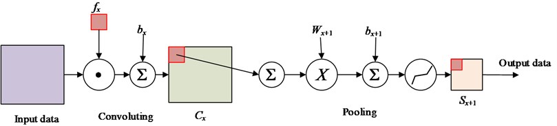
The convolutional neural networks generally contain input layer, convoluting layer, pooling layer and output layer, as illustrated in Fig. 1. As an end-to-end learning method, it can autonomously learn the representations of the data by their layer structure [28]. According to the convoluting theory, the feature maps of previous layer convolve with learnable kernels and put through the non-linear activation function, such as sigmoid, tanh, ReLU functions [29], to form the output feature mapping. Each output mapping integrates the convolutions with multiple input maps.

Fig. 1The schematic of convolutional neural networks

As a hierarchical architecture, inputting the arbitrary signal $x$, each subsequent layer $x_j$ is derived as:

2

$x_j=\rho W_j{x}_{j-1},$

where, the $W$ and $\rho$ are the linear operator and non-linear activation function, respectively. Typically, the $W_j$ is the convolution and $\rho$ is sigmoid $1/1+\mathrm{e}\mathrm{x}\mathrm{p}(-x)$ or rectifier $max(x,0)$ in convolutional neural networks. The operator $W_j$ is a stack of convolutional filters maps and each layer can be written as a sum of convolutions of the previous layer [30]:

3

$x_j\left(u,k_j\right)=\rho \left(\sum _k\left(x_{j-1}\left(\cdot ,k\right)\mathrm{*}{W}_{j,k_j}\left(\cdot ,k\right)\right)\left(u\right)\right),$

where, the * is the convolution operator:

4

$\left(f\mathrm{*}g\right)\left(x\right)=\sum _{u=-\mathrm{\infty }}^{\mathrm{\infty }}f\left(u\right)g\left(x-u\right).$

In convolutional neural networks, the optimization problem is highly non-convex. Typically, the weights $W_j$ are computed by stochastic gradient descent, by the backpropagation algorithm to compute gradients.

After the convolution layer, a pooling layer is followed and used to obtain the nonlinear down-sampling features [31]. This operation divides the input data into non-overlapping regions, and make the same operation ‘pooling’ for each region. The max-pooling function make the features to be a form of translation invariance and improve the computational efficiency of networks.

3. Methodology

3.2. Constructing the deep convolution neural networks (DCNN)

As one type of unsupervised neural networks, the sparse autoencode include the encoder and decoder, the former one transforms the input data from high-dimensional space into codes in a low dimensional space and the later one reconstructs the input from the corresponding codes. The autoencode with a hidden layer and linear output layer, which is the linear decode algorithm, is forced to learn a sparsity representation and reconstruct the original input.

The principle of CNN is very similar to the human’s visual processing and own the powerful performance in complex image identification. In the convolutional neural networks, the convoluting is the special filter method of feature extracting. The great innovation of convoluting and pooling layer is not full connect, so that the networks can extract the features, rather than fitting the input data.

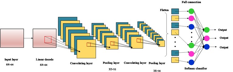
As the core of convolutional neural networks, the different deep learning model is constructed by the group of convoluting and pooling. The constructed DCNN model in this paper include one sparse aturoencode with linear decode layer, two convoluting layers, two pooling layers and a softmax layer. The schematic of DCNN is shown in Fig. 2. Because of the limitation of computational resource and efficient, the different time-frequency images must be shrunk the size by the nearest neighbor interpolation algorithm, and the pictures are normalized and centralized. Although many features would be eliminated by this method, the key features must be reserved and hardly effect the identification results. As the input data of DCNN model, all of these time-frequency images are 2-D feature and the size is 64×64. The advantage of this preprocess can survive the key features and release the computational performance.

Fig. 2The schematic of deep neural networks

Here, the neural networks architecture is detailly described as follows:

(1) In order to reducing the raw redundant of the input data, the original inputs are preprocessed by PCA whiten method, and the mean of inputs are zero. Besides, the sparse autoencode with linear decode algorithm is used to improve the sparsity of the input data as the first layer.

(2) Then, two convolutional layers with 8 feature maps are followed continuously. The kernels are selected and each kernel in feature maps is connected to a $p\times p$ neighborhood of input (here, the p is the patch dimension). The same kernel and connecting weights will be shared by the all neurons in one feature map.

In this process, the number of hidden neuron is initially estimated by the empirical formula Eq. (5):

5

$H_{\mathrm{n}\mathrm{u}\mathrm{m}}=\frac{n\times l+0.5\times (n^2+n)\times l-1}{n+l},$

where, $n$ is the dimension of features, $l$ is the number of fault classification.

(3) Following the each convoluting layer, the pooling layer with 4 feature maps are used with max-pooling operation. This operation can introduce the local translation invariance to the model and reduce the size of input data to the 1/4 compared with the previous convolution layer.

Fig. 3The flow chart of proposed method

(4) As a generalization of logistic function, the softmax can squashes a $K$-dimensional input vector of arbitrary real value to a $K$-dimensional output vector of real value in the range of (0, 1). It can efficiently solve multi-class problems. Therefore, a softmax layer with full connection is following the last pooling layer, and the output of the last pooling layer as the input of the softmax networks to obtain the identification and classification of the fault types from the time-frequency images efficiently.

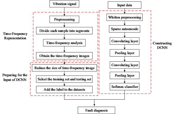
Based on the time-frequency representation and the constructed DCNN model, the flow chart of the fault feature extracting and classifying method is shown in Fig. 3. Although the STFT have limited time-frequency concentration and poor self-adaptability and affect the time-frequency representation, it does not affect the proposed DCNN model to identify the fault features obviously. Based on the DCNN model, the proposed method pretreats the input data by pre-whitening to eliminate the influence of relation and redundancy of input data, and the proposed model are constructed by the sparse decode and two convoluting layer and two pooling layer to strengthen the identifiability of fault information.

4. Experimental setup

As the key components of rotating machinery, the failure level and performance of rolling bearing and gear will greatly affect the reliability, service life and economic benefit of the machinery. Different kinds of faults will occur on the components under different working conditions. In this section, the proposed method is used to distinguish the fault features with the real testing vibration signals of fault bearing and gear. Simultaneously, some other existing methods such as CNN and LSSVM, which are already wildly used in fault diagnosis, are also used to compare their performance.

4.1. Case 1: Fault diagnosis of the rolling bearing

4.1.1. Data description

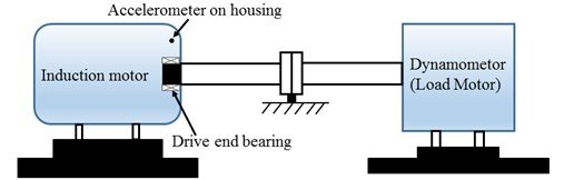
Here, the bearing fault data from the case west server university (CWSU) is used [32]. These data were collected from a bearing testing bed shown in Fig. 4. The single point faults of bearing components were produced to the testing bearing by electro-discharge with diameters 0.1778 mm, 0.3556 mm, 0.5334 mm, respectively. The loads of experiments were 0 hp, 1 hp, 2 hp and 3 hp, respectively. The vibration signals were collected by the accelerometers which were attached to the housing with 12000 samples per second. Here, the Normal condition (N), roller fault (RF), inner race fault (IF), outer race fault (OF) were selected under different fault diameters and loads. In this study, there are 200 signal samples under each fault conditions and each sample contain 4096 data points. The detailed of this strategy is shown in Table 1.

Fig. 4The schematic bearing testing bed

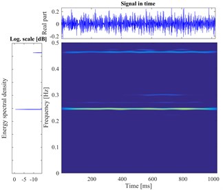
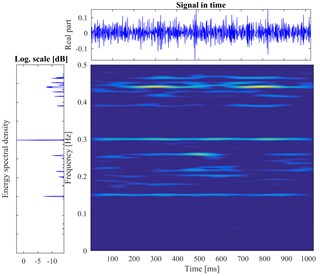
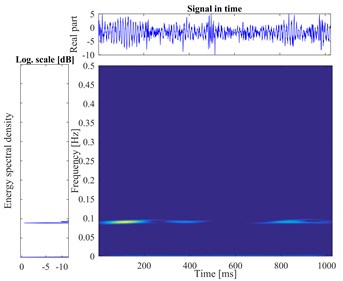
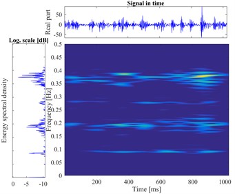
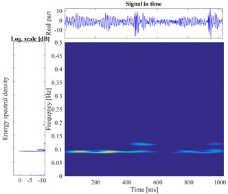
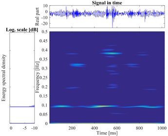
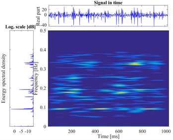
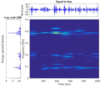
According to the proposed method, The STFT is performed to every segmented signal in all samples and the total of 800 different time-frequency images are obtained. There are divided into training sets and testing sets with the labels. The datasets as the input of the proposed DCNN model to perform the fault identification. The segmental vibration signals and the time-frequency pseudo-color maps of roller bearing are shown in Fig. 5. Here, the load is 3 hp and the diameters of faults are 0.1778 mm, 0.3556 mm, 0.5334 mm, respectively. In each picture, the upper waveform is the collected vibration signal and the left one is the power spectrum of the signal. The time-frequency representation through the STFT method is in the middle and the frequency is normalized. The sampling frequency is 1024, and the visualization threshold of time-frequency energy distribution on the images is 2 %, which can excellently display the detailed energy distribution of time-frequency representation.

Table 1The detailed datasets of bearing faults

Load (hp)	Samples number	Defect Location	Defect diameter (mm)	Classification label
1-2-3	200-200-200	N	0	1
	200-200-200	RD	0.178	2
	200-200-200	RD	0.356	3
	200-200-200	RD	0.533	4
	200-200-200	ID	0.178	5
	200-200-200	ID	0.356	6
	200-200-200	ID	0.533	7
	200-200-200	OD	0.178	8
	200-200-200	OD	0.356	9
	200-200-200	OD	0.533	10

Fig. 5The vibration signal and the time-frequency pseudo-color map of roller bearing

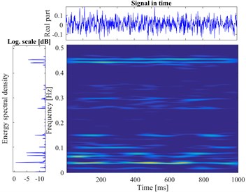
a) Normal bearing

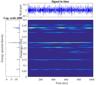
b) Ball fault in 0.1778 mm

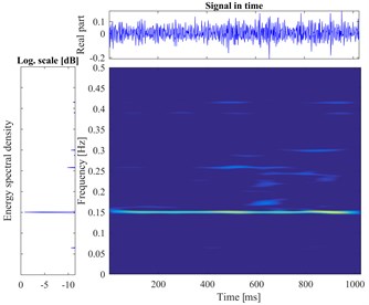
c) Ball fault in 0.3556 mm

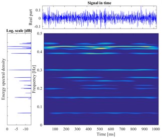
d) Ball fault in 0.5334 mm

e) Inner fault in 0.1778 mm

f) Inner fault in 0.3556 mm

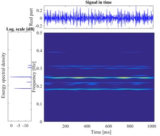
g) Inner fault in inch 0.5334 mm

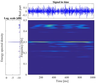
h) Outer fault in 0.1778 mm

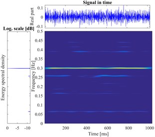
i) Outer fault in 0.3556 mm

j) Outer fault in 0.5334 mm

4.1.2. Diagnosis results

The initialized parameters of the bearing diagnostic model are listed in Table 2. In order to study the influence of the different key parameters on the proposed model, the influence of the key parameters on the classification accuracy of bearing faults are investigated. The number of hidden neurons, pooling dimensions, sparse parameter (desired average activation of the hidden units), batch size, the number of maximum iteration, different ratio of training samples and testing samples are selected to study. The number of hidden neuron has been determined by the Eq. (5). In this case, the $n$ is 64 and the $l$ is 10, and the hidden neuron is 290. The patch dimension and pooling dimension related to the input dimension, the former was the square root of 64, and the later one is the half of former. The number of maximum iteration and batch size are determined by the experience. And the other parameters, whiten parameter, weight decay, sparsity parameters, sparsity penalty, are determined as the constant according to the Ref. [19] and Ref. [20]. Here, the computer configuration is Inter i5-2430 and 16GB RAM in window 7 and Matlab 2016b.

Table 2The initialized parameters of bearing diagnosis model

Name	Value	Name	Value	Name	Value
Patch dimension	8	Pooling dimension	4	Whiten parameter	0.1
Hidden size	290	Weight decay	0.0003	Maximum iteration	200
Sparsity parameters	0.035	Sparsity penalty	5	Batch size	20

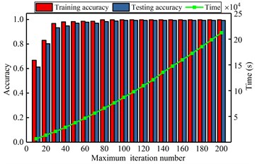
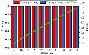
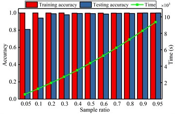
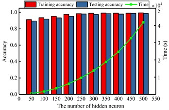
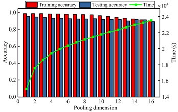
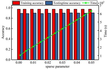
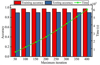
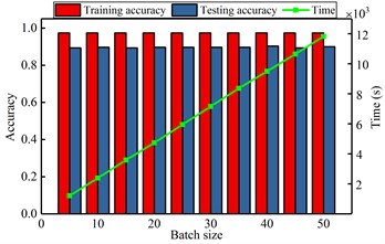
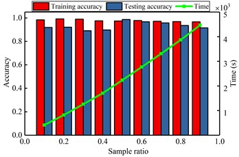
The computational results are shown in Fig. 6. Those figures show that the impact of selected key parameters on the computing accuracy and the exhausting time. From the Fig. 6(a), with the increasing of hidden neuron, the accuracy and time are both enlarged. When the number is greater than 220, the exhausting time is drastically increasing, but the accuracy is not significantly changing. It realizes that the optimal number of hidden neuron is 200 and the too large or too small number of hidden nodes will acquire the lower accuracy or too longer computational time. In the Fig. 6(b), it shows that the smaller pooling dimension can obtain the higher accuracy and less average time. Similarly, from the Fig. 6(c), (d), it can find that the minor sparsity parameter and the maximum iteration of sparse autoencoder have a lower accuracy and computing time. When the value is 0.02 and 60, respectively, it can achieve the satisfactory accuracy with suitable computing time. The bigger value will not improve the accuracy, instead of consuming more computational time. The Fig. 6(e), (f) show that the different batch and sample ratio have not significant effect to the classification accuracy. Oppositely, the bigger value consumes the more computational source. So, the appropriate values are 20 and 0.5.

Fig. 6The influence tendency of different parameters

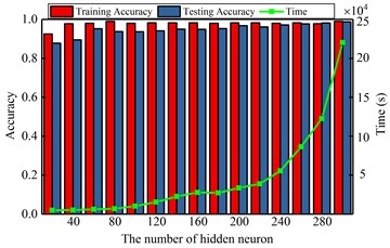
a) Diagnosis result by various the number of hidden neuron

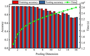
b) Diagnosis result by various pooling dimension

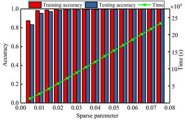
c) Diagnosis result by various sparse parameter

d) Diagnosis result by various maximum iteration number

e) Diagnosis result by various batch size

f) Diagnosis result by various sample ratio

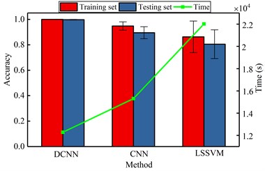
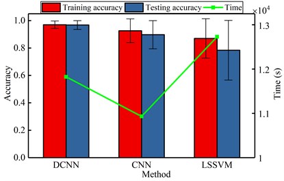
According to the analyzing, the optimal parameters are selected to perform the DCNN effectively, which are pooling dimension, sparse parameter, the number of hidden neuron, the number of iteration, batch size and sample ratio. When the DCNN model is training the bearing fault datasets, the classification accuracy of the training set and testing set are 100 % and 99.75 %, respectively, and the error is very small. The diagnosis results and the error are listed in Table 3 and the comparing results are shown in Fig. 7. From the Table 3 and Fig. 7, it shows that the proposed DCNN method have the smaller error and the more excellent performance. In our proposed model, the input data are pre-whitened and eliminated the correlation and redundancy. The sparse linear decode is used as the first layer of deep neural networks to decouple automatically and improve the sparsity of time-frequency images, these improved the identifiability of convoluting and pooling operating to extract the deep features. When the deep features of time-frequency images are obtained, the multi-class features are classified by the softmax layer accurately. And all of the parameters in the proposed DCNN model are optimized for fault diagnosis problem. So, the result of proposed method must have more excellent performance than CNN and LSSVM model.

Table 3The comparing of proposed method with other methods

	Proposed method	CNN	LSSVM
Training set accuracy	100 %	94.75 %	86.25 %
Testing set accuracy	99.75 %	89.50 %	80.50 %
Mean time	12276.3491	15310.3437	22013.821
Training set error	0	0.0328	0.124
Testing set error	0.0025	0.0471	0.1128

Fig. 7The histogram of comparative results for bearing

4.2. Case 2: Fault diagnosis of gears

4.2.1. Experiments and data description

The proposed method is used to diagnose the gear fault in this section. Six types of gear faults are investigated in this experimental case, which are normal condition, a single broken tooth of wheel, a single pit of wheel, a single worn of pinion, coupled fault of wheel pit and pinion worn, coupled fault of wheel broken and pinion worn. The vibration signals were collected on a specially designed bench which is driven by a motor. The detailed experiment illustration is shown in Fig. 8. The nominal power and speed are 0.75 KW and 1500 rpm, respectively. The pinion and wheel gear are located in the gearbox and their parameters are listed in Table 4.

Fig. 8The testing bed of gearbox

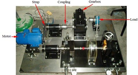
Table 4The parameters of gears

Gear	Teeth	Module (mm)	Pressure angle (deg)	Materials
Pinion	55	2	20	S45C
Wheel	75	2	20	S45C

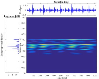
The time-frequency images of six types from the gear fault are displayed in Fig. 9, which load and rotational speed are 1 hp and 880 rpm, respectively.

Fig. 9The vibration signal and the time-frequency pseudo-color map of gear faults

a) Normal gear

b) Wear fault

c) Pit fault

d) Break fault

e) Pit and Wear compound fault

f) Break and Wear compound fault

4.2.2. Diagnosis results

In this case, the $l$ is 6 and the hidden neuron is 180. The determination method of other parameters are similar to the case 1. The initialized parameters of the DCNN model of gear fault diagnosis are listed in Table 5.

Table 5The initialized parameters of gear diagnosis model

Name	Value	Name	Value	Name	Value
Patch dimension	8	Pooling dimension	4	Whiten parameter	0.1
Hidden size	180	Weight decay	0.0003	Maximum iteration	200
Sparsity parameters	0.005	Sparsity penalty	5	Batch size	20

Fig. 10The influence of different key parameters

a) Diagnosis result by various the number of hidden neuron

b) Diagnosis result by various pooling dimension

c) Diagnosis result by various sparse parameter

d) Diagnosis result by various maximum iteration number

e) Diagnosis result by various batch size

f) Diagnosis result by various sample ratio

Here, the impacting of several parameters on the recognizing accuracy and computing time is studied in the gear fault diagnosis model. Similar to the bearing analysis, the number of hidden neuron, pooling dimension, sparse parameter, maximum iteration, batch size and sample ratio are selected. The detailed analyzing results are shown in Fig. 10. It shows that the number of hidden neurons and the ratio of samples have great influence on the diagnostic model. But the other parameters have stable effect on the model. When the different influence tendency of the parameters are determined, the optimal parameters are selected to diagnose the gear faults and the results are shown in Table 6 and Fig. 11. From the comparing results, it can significantly find that the proposed method has more excellent performance than other methods, not only for the computation accuracy, also for the efficiency. For the same reason in the case 1, it shows that the proposed DCNN model has more excellent performance than CNN and LSSVM model in the case 2.

Table 6The comparing of gear classification result

	Proposed DCNN	CNN	LSSVM
Training set accuracy	97 %	92.56 %	87 %
Testing set accuracy	96.78 %	89.72 %	78.33 %
Average time	11825.25	9032.3486	12730.4878
Training set error	0.0274	0.087	0.1334
Testing set error	0.0752	0.1035	0.2089

Fig. 11The histogram of gear fault classification result

5. Conclusions

In this work, a new intelligent fault diagnosis method of rotating machinery based on the time-frequency analysis and DCNN is proposed. The applicability and efficiency of the proposed method are verified by the collected vibration datasets of rolling bearing and gearbox with different fault characteristics. The conclusion of this work is summarized as follows:

1) Based on the convolutional neural networks, a new deep neural network called DCNN model is efficiently constructed with sparse autoencode, convoluting, pooling and softmax. This method integrates the sparse autoencode with linear decode method which can improve the sparsity of the input data and benefit to extract the fault features. The number of neurons and pooling dimension have great influence on the proposed DCNN model.

2) Because of the time-frequency representation contains more information of the fault feature than the time waveform or frequency spectrum, it is used as the new recognized object of proposed DCNN model. This method can extract the fault features without too many other transformations conveniently and precisely. The result show that the presented method can identify the different fault features from the time-frequency images and classify the fault conditions of the rotating mechanical effectively.

3) In the proposed method, the new application is advised, it not only works for the fault diagnosis of rotating mechanical whose measured signals are periodic, can also use to the other non-periodic vibration signals. In practice, the priori knowledge and fault data were hard to obtain, but many fault information still could collect to train the proposed DCNN model to verify the real fault features. In addition, the normal and fault condition of rotating components must be distinguished by the proposed model. After it was trained, the proposed model would be used to detect the fault types.