A method for analyzing the revolute joint wear of planar multibody systems and its application in unbalance loading working condition

Lai, Xiongming; Liu, Yisheng; Ji, Tianchen; Wang, Cheng; Zhang, Yong

doi:10.21595/jve.2018.18979

Journal of Vibroengineering

Browse Journal

Submit article

Published: 30 September 2018

Check for updates

A method for analyzing the revolute joint wear of planar multibody systems and its application in unbalance loading working condition

Xiongming Lai¹

Yisheng Liu²

Tianchen Ji³

Cheng Wang⁴

Yong Zhang⁵

¹Fujian South Highway Machinery Co., Ltd, Quanzhou, Republic of China

^{1, 2, 3, 5}College of Mechanical Engineering and Automation, Huaqiao University, Xiamen, 361021, Republic of China

⁴College of Computer Science and Technology, Huaqiao University, Xiamen, 361021, Republic of China

Corresponding Author:

Yisheng Liu

Cite the article Download PDF

Downloads 1490

WoS Core Citations 1

CrossRef Citations 1

Abstract

This paper develops an efficient method to describe the evolution of the revolute joint wear during the process of the mechanism movement. In the framework of multibody systems formulation, the prediction method of the revolute joint wear in different motion time interval is established by considering the wear ranges between the pin and the bushing on the basis of the Archard’s wear model. Then a typical non-planar mechanism with unbalancing loads acting on single non-ideal revolute joint is used to illustrate the application of the method. Moreover, the corresponding experimental mechanism is tested to validate the predicting results of the proposed method. The analysis shows that the method proposed is of high efficiency and can guarantee enough predicting accuracy when the predicted wear depth is not big. Therefore, the method is practical to a certain degree in engineering.

1. Introduction

Revolute joint is the most common pair for mechanism links. In mechanism movement where the relative slide and applied loads always exist between the pin and bushing within a revolute joint, the revolute joint wear is inevitable [1-9]. As the wear increases, the clearance size of the revolute joint increases as well, which results in the kinematic and dynamic degradation in the mechanism [10-12]. Therefore, it is necessary to study the evolutionary process of revolute joint wear in mechanism movement.

Studies on revolute joint wear mainly include two aspects: firstly, establishing a computational method for considering the immediate influence of revolute joint clearance and secondly, calculating gradually changes of the revolute joint clearance wear. Early studies focused on simple methods to obtain insight into the behavior of systems with joint clearances., including the spring-damper approach proposed by Dubowsky [13] and the massless link approach proposed by Earles and Wu [14]. Among them, the concept of a massless link has attracted the attention of many researchers due to its simplicity and has been used in studies like vibration and noise of mechanisms caused by joint clearance [8], the clearance contact loss in mechanisms [15], link size optimization with joint clearance accounted [16] and vibration analysis [17-19].

However, these methods are too simple to consider enough factors and cannot describe the contact-impact phenomenon in mechanism clearance. Later, more complicated clearance theories are developed for researching the behavior of systems with joint clearances. Overall, the complicated clearance theories can be divided into two types, that is, the discontinuous method and the continuous one [5]. The discontinuous method assumes that the period of the impact is very short, and the configuration of the system doesn’t change. Though adopted by many scholars [20-22], the fact that the duration of the impact process is unknown has restricted its application. The continuous method [23] assumes that the forces and penetrations between the pin and the bushing vary continuously. The method adopts the continuous contact force model to calculate the forces during the impact and sliding process. In recent years, the idea of the continuous contact-impact conception has been widely applied [24-26], with various continuous contact force models developed successively, such as Kelvin-Voigt model [27], Hertz model [28], Lankarani-Nikravesh mode [24] and so on. In particular, the impact force in Lankarani-Nikravesh model takes both the influences of impact deformation and damping hysteresis effect; therefore, it provides a good description of energy dissipation in the course of contact. All in all, great progress has been made in this field.

Unlike great deals of works referring to joint clearance research, there have been encountered only a few studies addressing the issue of the joint clearance wear. Currently, Reye’s hypothesis [29] and the Archard’s wear model [23, 30] are the most popular ways to calculate wear. The Reye’s hypothesis tells that, in the case of dry friction, the volume of removed material is proportional to work performed by the friction forces. As far as the Archard’s wear model is concerned, it correlates the wear volume with some physical and geometrical properties of the sliding bodies, such as applied load, sliding distance and hardness. Relatively speaking, Archard’s approach takes more factors into account compared to Reye's approach and the former corresponds with the reality to a larger extent. Researches on revolute joint wear with the Reye’s hypothesis is relatively less [31]. Most scholars tend to use the Archard's wear model for revolute joint wear researches. P. Flores developed a method for studying and quantifying the wear phenomenon in revolute clearance joints [32]. In his method, the surfaces of the pin and bushing are divided into several sectors to perform the wear analysis. Firstly, each contact sector of the pin and bushing is obtained by the multibody system simulation within each time step. Then by means of the contact conditions obtained from the simulation, the radii of the pin and bushing corresponding to each sector are modified as the wear results. Saad Mukras et al. incorporated the finite element analysis into the multi-body dynamic system [33, 34]. In their method, the finite element method is responsible for the joint wear analysis and the multi-body dynamic system for obtaining the contact condition. Then the joint wear evolved in the mechanical system can be predicted. Bai et al. used the similar method to study the wear phenomenon of clearance joint in the planar mechanical system. Their modification is that the action forces in joint contact analysis is different [3]. In their another work, they pointed out that their modified model for the joint action forces had a greater applicable scope [9].

However, researches mentioned previously are faced with the problem of excessive computation. Usually, the wear of mechanism revolute joint clear evolves slowly. Correspondingly, the wear of the mechanism in a single motion period is too small; therefore, the wear only becomes countable when thousands of motion periods of the mechanism movement are simulated. In each motion period of mechanism movement simulated in Ref. [33], Ref. [34] and Ref. [9], the finite element method has been applied to simulate the contact wear process of the pin and the bushing in order to calculate the wear amount. Therefore, their methods are too time-consuming to calculate mechanism movement of thousands of motion periods and are not suitable for the practical engineering applications. Adopting a more direct method rather than the finite element method, Ref. [32] involves less calculation load than the former. In this paper, a new method for calculating revolute joint wear is proposed, which is believed to be more efficient than the method in Ref. [32] because the wear depth only needs to be calculated once for every single motion period rather than calculated once for each corresponding time step in a single motion period. Besides, the methods adopted in the previous literatures are merely used for numerical simulations without being verified by experiment and their effectiveness is still unknown. Therefore, in this paper, the wear tests of the experimental mechanism have been further used to verify the presented method and discuss its effectiveness and efficiency.

Moreover, due to the need of assemblage, the experimental mechanism is non-planar, i.e. their links are not coplanar. This cause unbalancing loads acting on the revolute joint in the experimental mechanism. Obviously, this factor is ubiquitous in practical engineering mechanisms. Presently, there are no literatures on the joint wear with such factor considered. However, this paper will consider this important factor when using the presented method to predict the revolute joint wear. Further, the prediction results will compare with the experimental results to show practicability of the presented method for practical engineering mechanisms.

2. The modeling of multibody dynamic system with clearance

The modeling of multibody dynamic system with clearance can be divided into two parts: The model of multi-body dynamic system and the clearance contact model.

2.1. Multibody dynamic system model

The multi-rigid-body system refers to the complicated mechanical system composed of multiple rigid bodies connected by kinematic pairs. The multi-rigid-body system dynamics, currently a mature theoretical method, focuses on the motion law of the multi-rigid-body system. In Cartesian coordinate system, the unconstraint equation of motion in the multi-body system can be written as:

1

M {\ddot{q}}_{} = g,

where $q = [{q_{1}}^{T}, {q_{2}}^{T} . . ., {q_{i}}^{T} . . ., {q_{n}}^{T}]^{T}$ is the generalized matrix composed by the generalized coordinates of all the rigid bodies. $M$ refers to the mass matrix composed by the mass of all the rigid bodies. $M_{i}$ is the mass of Rigid body $i$ . $g$ is the generalized force vector composed by the generalized force of all the rigid bodies including the external force and the Coriolis force on the rigid bodies. $g_{i}$ is the generalized force acting on Rigid body $i$ .

For the unconstraint multi-body system, the kinematic pairs equal the following algebraic constraint equations:

2

Φ (q, t) = 0 .

In the following paper, $Φ (q, t)$ is abbreviated as $Φ$ . By use of Lagrangian Multiplier, the constraint equation above can be added into the equation of motion; then the equation of the multi-rigid-body system can be deduced:

3

[\begin{matrix} M & Φ_{q}^{T} \\ Φ_{q} & 0 \end{matrix}] [\begin{array}{l} \ddot{q} \\ λ \end{array}] = [\begin{array}{l} g \\ γ \end{array}],

where $λ$ refers to Lagrangian Multiplier vector. $γ$ is the acceleration item that is only related to the velocity, which can be expressed as follows:

4

γ = - (Φ_{q} \dot{q})_{q} \dot{q} - Φ_{t t} - 2 Φ_{q t} \dot{q}

where $Φ_{t}$ denotes the first derivative of $Φ$ with respect to time $t$ . $Φ_{t}$ denotes the second derivative of $Φ$ with respect to time $t$ . $Φ_{q t}$ denotes the derivative of $Φ$ with respect to both time $t$ and $q$ .

Eq. (4) is the differential-algebra equations that need to be solved. The equation can also be called Euler-Lagrange Equations. Refer to [35-36] for more information.

2.2. Clearance model

2.2.1. Description of clearance contact model

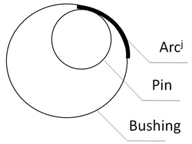
In Fig. 1, the pin circle connecting with Rigid body $i$ represents the pin, while the bushing circle connecting with Rigid body $j$ represents the bushing. $O_{i}$ and $O_{j}$ are the axes of the pin and bushing, respectively. $R_{i}$ refers to the radius of the pin, while $R_{j}$ the radius of the bushing. The clearance size is $c = R_{i} - R_{j}$ . When the pin and bushing do not contact each other, there are no force constraints between them; but when they are contacting each other, a contact force will be generated, in which case the model of force constraints must be introduced for description and reflected in the mechanics equation of the multi-rigid-body system.

Fig. 1Revolute joint with clearance

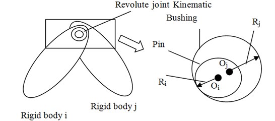
Fig. 2Pin and Bushing contact each other

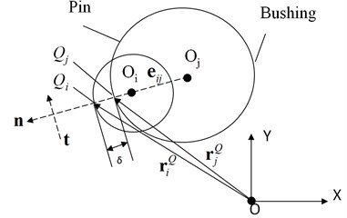
Fig. 2 shows that the pin and the bushing are contacting each other. $O$ refers to the global origin of coordinates. $X$ - $Y$ represents the global coordinate system. $r_{i}^{O}$ and $r_{j}^{O}$ refer to the positions of the pin and the bushing in global coordinate system. The eccentric vector of the pin and the bushing is $e_{i j}$ which can be shown as below:

5

e_{i j} = r_{j}^{O} - r_{i}^{O} .

The module of eccentric vector $e_{i j}$ equals the eccentric distance $e_{i j}$ . The unit normal vector is $n$ . $e_{i j}$ and $n$ can be written as the below:

6

e_{i j} = \sqrt{e_{i j}^{T} e_{i j}},

7

n = \frac{e_{i j}}{e_{i j}} .

Fig. 2 describes the collision between the pin and the bushing. The two contact points, $Q_{i}$ and $Q_{j}$ belong to the pin and the bushing, respectively. The positions of $Q_{i}$ and $Q_{j}$ can be described by position vectors $r_{i}^{Q}$ and $r_{j}^{Q}$ in global coordinate system. The penetration depth $δ$ is the distance between the two contact points and it can be described as:

8

δ = e_{i j} - c .

In the model of the multi-body dynamic system, the velocities of the two contact points in global coordinate system can be figured out. The velocities can be assumed as ${\dot{r}}_{i}^{Q}$ and ${\dot{r}}_{j}^{Q}$ . The relative velocity of the contact points $Q_{i}$ and $Q_{j}$ , including the normal component and the tangential component, can be given by:

9

ν_{N} = ({\dot{r}}_{j}^{Q} - {\dot{r}}_{i}^{Q})^{T} n,

10

ν_{T} = ({\dot{r}}_{j}^{Q} - {\dot{r}}_{i}^{Q})^{T} t .

The unit tangential vector $t$ can be obtained by rotating the unit normal vector $n$ by 90° in the anti-clockwise direction.

2.2.2. Calculation of clearance force

Clearance force includes the normal contact force and tangential friction force. Firstly, the calculation of the normal contact force is the key to simulating interactions between the pin and bushing. Apparently, the impact velocity, physical material properties, the geometry characteristics of the contacting bodies and the deformation all have influence on the contact force; that’s why all these factors must be taken into account. Based on the work of Hunt and Crossley [37], Lankarani and Nikravesh [24] proposed that besides the impact deformation, the damping hysteresis effect must be taken into account in order to better describe the energy dissipation in the course of contact. The normal contact force model equation is expressed as:

11

F_{N} = K^{'} δ^{n} + K^{''} \dot{δ},

where the first term indicates the elastic force, while the second one refers to the energy dissipation. $K^{'}$ denotes the stiffness coefficient of the impact body. $δ$ represents the penetration depth. $n$ is the exponent, related to the material of contact and impact. $\dot{δ}$ refers to the relative deformation velocity. The stiffness coefficient $K^{'}$ depends on the material characteristics and the geometric characteristics of the colliding bodies. $K^{'}$ can be described with the following equation:

12

K^{'} = \frac{4}{3 π (h_{i} + h_{j})} {(\frac{R_{i} R_{j}}{R_{j} - R_{i}})}^{1 / 2},

13

h_{k} = \frac{1 - ν_{k}^{2}}{(π E_{k}) k} = i, j,

where $ν_{k}$ and $E_{k}$ refer to Poisson’s coefficient and Young modulus, respectively. For general steel, $ν_{k}$ and $E_{k}$ can be set as 0.3 and 207 MPa.

$K^{''}$ is the damping coefficient, and can be given as follow [38]:

14

K^{''} (δ, d_{m a x}, C_{m a x}) = \{\begin{array}{l} 0, & δ \leq 0, \\ C_{m a x} {(\frac{δ}{d_{m a x}})}^{2} (3 - \frac{2 δ}{d_{m a x}}), & 0 < δ < d_{m a x}, \\ C_{m a x} & δ \geq d_{m a x} . \end{array}

In Eq. (17), $d_{m a x}$ is the maximum penetration depth. $C_{m a x}$ is the maximum damping coefficient. According to the previous research [38], the value of $d_{m a x}$ is 0.01; while $C_{m a x}$ is generally 1 % of the stiffness coefficient $K^{'}$ .

Shivawamy [39] has demonstrated, theoretically and experimentally, that in the low velocity case, the damping hysteretic effect is the main factor that causes energy dissipation. If the velocity is high, the energy dissipation will be caused by other factors which are not included in the Eq. (14). Since this paper focuses on the low velocity mechanism, this model used here is suitable for describing the clearance contact force in the paper.

In order to enhance the applicability of the clearance contact model, the widely used Coulomb friction model is also applied here, as illustrated below:

15

F_{f} = \frac{μ F_{N} ν_{T}}{‖ν_{T}‖},

where $μ$ is the friction coefficient and it can be obtained through the experiment introduced by Schmitz and others [40].

In the analysis of the multi-body dynamics, many researchers have adopted the model of clearance impact force as shown in Eq. (14). The model can well describe the nonlinear characteristics of clearance impact.

3. A new high efficient method for predicting revolute joint wear

3.1. Calculation of the wear depth of revolute joint

Currently, several methods of predicting wear have been developed, among which the Archard’s wear model developed on the basis of test is the most widely used [33, 41-43]. The model links the wear volume, sliding distance and hardness, which is shown as follows [30, 41]:

16

\frac{V}{S} = \frac{K}{H} F_{N},

where $V$ stands for the wear volume. $S$ is the sliding distance. $K$ is the wear coefficient. $H$ is the hardness of materials. Further, dividing Eq. (19) by $A_{a}$ , the actual contact area results in:

17

h = \frac{K}{H A_{a}} F_{N} S,

where $h$ is the wear depth.

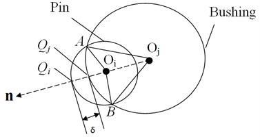
As for the clearance collision model studied in this paper, when the penetration depth corresponding to the pin and bushing is $δ,$ $|O_{j} Q_{i}| = R_{j} + δ,$ $|O_{j} Q_{j}| = |O_{j} A| = |O_{j} B| = R_{j},$ $|O_{i} A| = |O_{i} B| = |O_{i} Q_{i}| = R_{i}$ and $|O_{j} O_{i}| = R_{j} + δ - R_{i}$ are obviously tenable, as is shown in Fig. 3. In $Δ O_{j} O_{i} B$ :

18

θ = ∠ O_{i} O_{j} B = a r c c o s (\frac{{|O_{i} O_{j}|}^{2} + {|O_{j} B|}^{2} - {|O_{i} B|}^{2}}{2 |O_{i} O_{j}| |O_{j} B|})

= a r c c o s [\frac{(R_{j} + δ - R_{i})^{2} + {R_{j}}^{2} - {R_{i}}^{2}}{2 (R_{j} + δ - R_{i}) R_{j}}] .

In $Δ O_{j} A B$ :

19

|A B| = \sqrt{{|O_{j} A|}^{2} + {|O_{j} B|}^{2} - 2 |O_{j} A| |O_{j} B| c o s (2 θ)} = \sqrt{2 {R_{j}}^{2} [1 - c o s (2 θ)]} .

Furthermore:

20

A_{a} = |A B| * w,

where $w$ is the contact width between the pin and bushing.

By simultaneous Eqs. (17)-(20), the wear depth $h$ can be calculated.

Fig. 3Calculation of the contact length when the pin and bushing collide

3.2. Calculation of wear depth of revolute joint with wear ranges considered

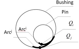
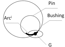
In Fig. 4, $A r c^{i}$ and $A r c^{j}$ refer to the ranges of the pin’s and the bushing’s contact points $Q_{i}$ and $Q_{j}$ , respectively.

Fig. 4The ranges that the contact point between the pin and the bushing covers on their verges within single motion period

In this paper, the previously established mechanism model that involves revolute joint model can be used to determine the wear ranges $A r c^{i}$ and $A r c^{j}$ as well as the collision information corresponding to any time t within the range, including sliding velocity $V (t)$ , normal collision force $F_{N}^{} (t)$ , contact arc length $A B (t)$ and contact area $A_{a}^{} (t)$ . For the convenience of calculation, the normal collision force $F_{N}^{} (t),$ contact arc length $A B (t)$ and contact area $A_{a}^{} (t)$ are approximately considered as equal everywhere within the ranges of $A r c^{i}$ and $A r c^{j}$ , that is, $\bar{F_{N}}$ , $\bar{A B}$ and $\bar{A_{a}}$ . Therefore, according to Eq. (17), the wear depth in the pin wear range $A r c^{i}$ can be considered as equal everywhere. Similarly, the wear depth in the bushing wear range $A r c^{j}$ is also considered equal everywhere. Then, in this motion period, the sliding distance $S$ between the two plane circles in the joint clearance model, average normal collision force $\bar{F_{N}}$ , average contact arc length $\bar{A B}$ and average contact area $\bar{A_{a}}$ can be given by:

21

S = \int_{0}^{T} |V (t)| d t,

22

\bar{F_{N}} = \frac{1}{T} \int_{0}^{T} F_{N} (t) d t,

23

\bar{A B} = \frac{1}{T} \int_{0}^{T} A B (t) d t,

24

\bar{A_{a}} = \frac{1}{T} \int_{0}^{T} A_{a} (t) d t .

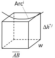
Fig. 5Calculating the wear volume of the bushing in single motion period

a)

b)

Suppose the wear range of the bushing is not $A r c^{j}$ (see Fig. 4) but is restricted at the local point G (see Fig. 5(a)). Then according to Eqs. (17)-(20), the bushing’s wear depth $Δ h_{j}^{*}$ at the local point G can be calculated as long as all the information including the sliding distance $S$ , the normal clearance collision force $\bar{F_{N}}$ , the contact arc length $\bar{A B}$ and the contact area $\bar{A_{a}}$ are known:

25

Δ h_{j}^{*} = \frac{K^{j}}{H^{j} \bar{A_{a}}} \bar{F_{N}} S,

where $K^{j}$ and $H^{j}$ refer to the wear coefficient and hardness of the bushing, respectively.

Fig. 5(b) enlarges the local point G. The cube is the wear volume of the bushing at the local point G and obtained by:

26

V_{v o l u m e}^{j} = \bar{A B^{}} \times w^{} \times Δ h_{j}^{*} .

Actually, the wear range of the bushing is $A r c^{j}$ rather than being restricted in the local point G. Therefore, the wear volume $V_{v o l u m e}$ at the local point G should be distributed to the wear range $A r c^{j}$ . The volume after distributing should be consistent to $V_{v o l u m e}$ , that is:

27

V_{d i s t r i b t u e}^{j} = V_{v o l u m e}^{j} .

The average wear depth in the whole wear range $A r c^{j}$ can be further deduced as:

28

Δ h_{j} = \frac{V_{d i s t r i b u t e}^{j}}{L_{a r c}^{j} \times w} = Δ h_{j}^{*} \times \frac{\bar{A B}}{L_{a r c}^{j}},

where $L_{a r c}^{j}$ refers to the length of $A r c^{j}$ .

Considering both Eqs. (25) and (28), the average wear depth of the bushing in the wear range $A r c^{j}$ is rewritten as:

29

Δ h_{j} = \frac{\frac{K^{j}}{H^{j} w} \bar{F_{N}} S}{L_{a r c}^{j}} .

Similarly, the average wear depth of the pin in the wear range $A r c^{i}$ can also be calculated through the following equation:

30

Δ h_{i} = \frac{K^{i}}{H^{i} w} \bar{F_{N}} S \times / L_{a r c}^{i} .

At last, in a single motion period, the wear depth of the revolute joint equals the sum of the pin’s and the bushing’s wear depths:

31

Δ h = Δ h_{i} + Δ h_{j} .

It should be noted that in case of mechanisms with low velocity, the pin and the bushing in a revolute joint continuously contact each other and the wear ranges in every motion period are basically the same; therefore, the wear ranges $A r c^{i}$ and $A r c^{j}$ of every motion period are also the same. However, in case of mechanisms with high velocity, there are three configurations of the joint components (i.e. the pin and bushing) [30]: free-flight motion, the impact condition and the sliding condition. And the contact position differs a lot in every motion period; therefore, the contact wear range $A r c^{i}$ and $A r c^{j}$ of different motion periods differs a lot. In other words, the clearance wear calculation proposed in this paper only applies to mechanisms with low velocity.

3.3. The prediction method of revolute joint wear in different motion time intervals

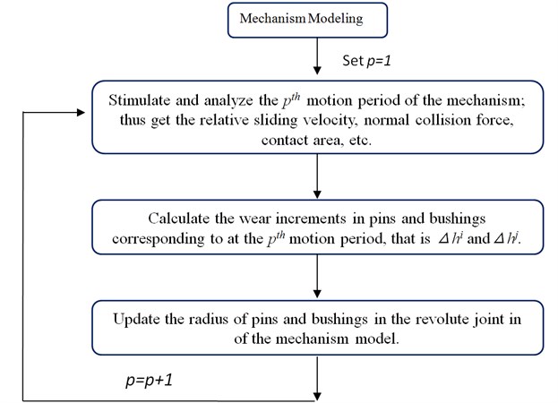
Fig. 6 shows the common way of computing the wear increment of revolute joint in each motion period. Usually, during the service life of mechanisms, there are quite a lot of motion periods. Fig. 6 provides a method to study the evolution of revolute joint wear during its service life by simulating mechanism movement one motion period by another, but the method involves too much calculation which is time-consuming and is not suitable for engineering applications.

Fig. 6Calculating the revolute joint wear depth one motion period by another

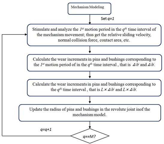
Therefore, in order to improve the computation efficiency, it is feasible to calculate the wear increment of the revolute joint one-time interval by another. It is supposed that the overall operating time corresponding to the service life of the mechanism is $T_{t o t a l}$ , which is divided into $M$ time intervals and each time interval includes $L$ motion periods. Refer to Fig. 7 for the detailed computation process. The wear increments of each motion period in each interval are basically the same if the selected $M$ and $L$ are proper. Therefore, the wear increment of the revolute joint in each time interval can be approximately got by calculating the increment in a motion period once. In this way, the computation efficiency can be greatly improved.

Usually, revolute joint wear includes three stages: running-in wear, stable wear and severe wear. During the stable wear stage, the wear condition and its resulting wear of the revolute joint are stable. Therefore, when applying the above method, it is advisable to predict the wear within the stable wear stage for the prediction accuracy.

Fig. 7Calculating the wear depth of the revolute joint within one-time interval by another

4. Numerical example and experimental validation

In this section, the non-planar four-bar mechanism with unbalanced loads acting on single non-ideal joint clearance is used as examples to demonstrate the wear prediction of the proposed method and the related experimental test is carried out to validate the correctness of the predicted results.

4.1. Experimental mechanism introduction

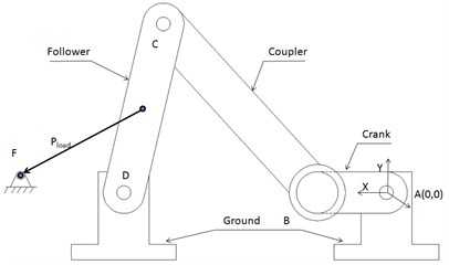
Fig. 8(a) shows the diagram of the non-planar four-bar mechanism. Its Revolute joint B is non-ideal and Revolute joint A, C and D are ideal ones. Fig. 9 is the corresponding the wear test-bed of the four-bar mechanism. All bars of the mechanism are made of Steel No. 45, with their geometric and inertial parameters shown in Table 1. The test aims to measure the wear of Revolute joint B. The pin and the bushing in Revolute joint B are connected to the crank and the connecting rod, respectively. To enhance the wear effects, the bushing is made of 1060 aluminum and the pin is made of Steel No. 45. Since the hardness of the two materials differs a lot, the wear on the surface of the pin can basically be considered as null and can thus be ignored. On the other hand, the bushing is made of soft materials, with considerable wear losses obtained in a short period of time. The initial radius of the pin and the bushing is 9.9 mm and 10.0 mm, respectively. The initial clearance size is thus 0.1 mm. Table 2 is a detailed list of the sizes and materials of the pin and the bushing in Revolute Joint B. Besides, pins and bushings of Revolute joint A, C and D are all made of Steel No. 45. Compared with the wear of Revolute joint B, the wear of Revolute joint A, C and D are too small to be counted. Therefore, Revolute joint A, C and D are deemed as ideal and Revolute joint B as not ideal in the wear test-bed of the four-bar mechanism.

Besides, Fig. 8(b) is the local enlargement of Revolute joint B. The crank and the coupler are not on the same plane. Hence, the four-bar mechanism is non-planar. C₁ and C₂ are the contact points between the pin and the bushing. Most of time, the direction of their acting forces, i.e. Force₁ and Force₂, are out of plane. Naturally, Revolute Joint B bears unbalanced loads. And such consideration corresponds with the reality to a larger extent. As a result, the mechanism in Fig. 8 is called the non-planar mechanism with unbalanced loads for short.

Fig. 8The non-planar four-bar mechanism with unbalanced loads acting on non-ideal joint clearance

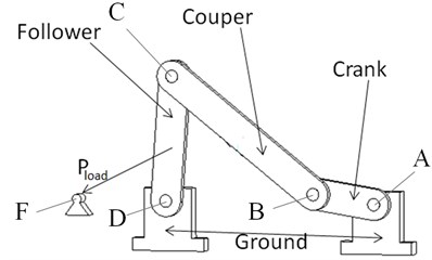
a) The diagram of the non-planar four-bar mechanism with a non-ideal revolute joint

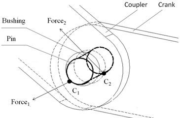
b) Local enlargement of Revolute joint B

Fig. 9The wear test-bed of the four-bar mechanism

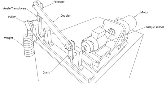
Table 1The geometric and inertial parameters of the four-bar mechanism

	Length (m)	Mass (kg)	Inertia (kg·m²)
	Length (m)	Mass (kg)	$I_{x x}$	$I_{y y}$	$I_{z z}$
Crank	0.1	0.4973	7.796×10^-4	8.801×10^-4	1.088×10^-4
Coupler	0.35	1.479	1.784×10^-2	1.814×10^-2	3.214×10^-4
Follower	0.25	1.086	7.189×10^-3	7.407×10^-3	2.363×10^-4
Ground	0.37

Table 2The sizes and materials of the pin and the bushing in Revolute Joint B

Initial bushing radius	10.0 mm
Initial pin radius	9.9 mm
Pin-bushing width	20.0 mm
Young’s module of 304 stainless steel	2.04×10¹¹N/mm²
Poisson’s ratio of 304 stainless steel	0.285
Young’s module of 1060 aluminum	6.9×10¹⁰N/mm²
Young’s module of 1060 aluminum	0.33
Hardness of 1060 aluminum	21 HB

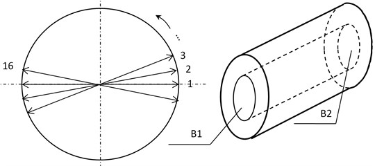
Point A in the mechanism is the global coordinate origin, and the crank, which is the driving link, rotates Point A with a constant angular velocity of 9.6 r/min. Point E is at the center of the follower. In the process of the mechanism motion, there is a load $P_{l o a d}$ (= 101.92 N) that always points to Point F. The crank is initially placed in a horizontal position, and the pin in Revolute Joint B is concentric with the bushing. The mechanism will operate for 88 hours, during which the diameter of the bushing on the circumferential side (B1 and B2) will be measured every two hours as indicated in Fig. 10. By doing so, the wear depth variations corresponding to each part of the bushing can be collected.

Fig. 10The measurement of the diameter of the bushing in Revolute Joint B

4.2. Analysis of wear range

Fig. 11 shows the wear of Side B1 and Side B2 in Revolute Joint B after 88 hours. A few points are worth to be paid attention: (1) The wear on Side B1 are more severe than that on Side B2, which indicates that the loads on Side B1 is heavier than those on Side B2. (2) The wear ranges on Side B1 and Side B2 are both located on the upper part of the bushing. (3) The wear ranges on Side B1 and Side B2 can be divided into two parts (see Fig. 11). The first part is within the range of angle $β$ and the second part is within the range of angle $φ$ . Since the wear depth within the angle range $φ$ is significantly greater than that within the angle range $β$ , the main wear areas are therefore focused within the angle range $φ$ . Moreover, it can be inferred that the wear of Side B1 and Side B2 at any moment during the 86 hours is similar to what is demonstrated in Fig. 11. That is, the wear areas are mainly focused within the angle range $φ$ during the whole wear process.

Fig. 11The wear of Side B1 and Side B2 in Revolute Joint B after 88 hours

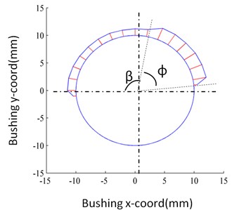
a) Side B1

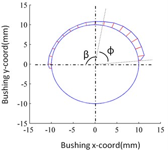
b) Side B2

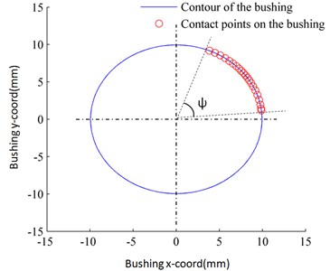
Two plane circles are used to simulate the clearance collision between the bushing and the pin in this paper. Therefore, the crank and the connecting rod that connect the pin and the bushing, respectively, should be on the same plane. To do that, the planar four-bar mechanism in Fig. 12 is adopted to simulate the wear of the non-planar mechanism with unbalanced loads in Fig. 8. The bushing and the pin of Revolute joint B in Fig. 8 are replaced by two plane circles (see Fig. 12), and the crank and the coupler in Fig. 12 are on the same plane. The distribution of the contact points ( $ψ$ ) on the bushing in Revolute Joint B can be measured through a numerical analysis of the planar four-bar mechanism with single clearance model (see Fig. 13).

Fig. 12The planar four-bar mechanism with balanced loads acting on joint clearance

It is worth noting that the wear range in Fig. 11 is wider than that in Fig. 13, for the use of two plane circles in simulating the clearance collision cannot take into consideration the impact of unbalanced loads. Nevertheless, the distribution of contact points within the angle $ψ$ in Fig. 13 remains basically the same as the main wear range that limited in the angle $φ$ shown in Fig. 11. Therefore, it is feasible to use a planar four-bar mechanism with a single clearance model to simulate and predict the wear of Revolute Join B of the mechanism with unbalanced loads.

Fig. 13The distribution of the contact point of the bushing of Revolute joint B simulated by the planar four-bar mechanism with single non-ideal clearance shown in Fig. 12

The distribution of the contact point of the bushing of Revolute joint B simulated by the planar four-bar mechanism with single non-ideal clearance shown in Fig. 12

4.3. The calculation of equivalent wear coefficient

As shown in Fig. 11, the wear extents on Side B1 and Side B2 differ due to the effect of unbalanced loads, which means that the wear conditions of Side B1 and Side B2 differ from each other. Using the planar mechanism shown in Fig. 12 and with reference to the different wear conditions of Side B1 and Side B2, the wear depths on the two sides are predicted, respectively. The crux of calculation is to obtain the equivalent wear coefficients of the two sides, respectively. Since the samples of the experiment, including the pin and bushing, have undergone a high-precision grinding and machining process, they enter the stable wear stage at the start of the wear test. Therefore, with part of the experimental data obtained in the early motion periods of the experimental mechanism, the equivalent wear coefficients can be derived.

Thus the Eq. (29) used to calculate the average wear depth of the bushing in each motion period is rewritten as follows:

32

Δ h_{j} = \frac{K^{j}}{H^{j} \bar{A_{a}}} \bar{F_{N}} S \times \frac{\bar{A B}}{L_{a r c}^{j}} .

Besides, the wear extent of Revolute joint B in the experimental mechanism is measured according to its average wear depth in the main wear range (see Fig. 11):

33

\begin{array}{l} h^{P} = \frac{1}{8} \sum_{m = 1}^{8} D_{m} - D_{0}, \\ Δ h^{P} = h^{P} - h^{P - 1}, \end{array}

where $D_{m}$ stand for the diameters of 8 points, which are uniformly distributed within the main wear range ( i.e. the wear area within the angle range $φ$ in Fig. 11); $D_{0}$ is the initial diameter of the bushing, that is 20.0 mm; $h^{p}$ is the cumulative wear depth after 2 $p$ hours; $∆ h^{p}$ is the wear depth increment after 2 $p$ hours.

Further, the average wear depth of the bushing in each motion period $Δ h_{j}$ is:

34

Δ h_{j} = \frac{Δ h^{P}}{M} .

Since the motion period of the experimental mechanism is 6.25 s, $M$ equals 1152 after two hours, that is, 1152 rounds. With Eqs. (32)-(34), the equivalent wear coefficient can be worked out.

By resorting to the cumulative wear depths measured from Side B1 and Side B2 in the first 10 hours of the operation of the experimental mechanism, the equivalent wear coefficients on the two sides are calculated (see in Tables 3-4).

Table 3Calculation results of the equivalent wear coefficients of the bushing on Side B1

Measure point	P0	P1	P2	P3	P4	P5	Mean value
Cumulative wear depth $h^{P}$ (mm)	0	0.0229	0.0496	0.0779	0.1000	0.1221	–
Increasing wear depth $∆ h^{P}$ (mm)	–	0.0229	0.0267	0.0283	0.0221	0.0221	–
Equivalent wear coefficients $K_{j}$ (10^-11 Pa^-1)	–	7.2992	8.5114	9.0665	7.0839	7.0981	7.8118

Table 4Calculation results of the equivalent wear coefficients of the bushing on Side B2

Measure point	P0	P1	P2	P3	P4	P5	Mean value
Cumulative wear depth $h^{P}$ (mm)	0	0.0159	0.0342	0.0538	0.0689	0.0841	–
Increasing wear depth $∆ h^{P}$ (mm)	–	0.0159	0.0183	0.01956	0.0152	0.0152	–
Equivalent wear coefficients $K_{j}$ (10^-11 Pa^-1)	–	5.0716	5.8303	6.2404	4.8549	4.8705	5.3735

Fig. 14The wear depth of the bushing of Revolute joint B in the four-bar mechanism uniformly distribute within the wear range

Obviously, the equivalent wear coefficients in Table 3 are larger than those in Table 4. It is because the wear depth of the bushing on Side B1 is larger than that on the Side B2; that is, the wear conditions are worse on Side B1.

It is noteworthy that the equivalent wear coefficients calculated through the above equations are not exactly equivalent to the actual wear coefficients of 1060 aluminum and 45# steel. It is because when the equivalent wear coefficients are calculated, it is assumed that the wear depth of the bushing is constant everywhere within the wear range $A r c^{j}$ (See in Fig. 14). But the actual wear depth of either the pin or the bushing is not uniformly distributed along the circumference. Due to the above difference, the wear coefficients obtained through the presented method are dissimilar from their actual value; thereby they are named the “equivalent wear coefficients”.

4.4. Wear prediction and verification

The planar mechanism in Fig. 12 is used to predict the wear of Side B1 of the bushing of Revolute joint B in the mechanism with unbalanced loads. The specific steps are as follows.

(1) With reference to the cumulative wear depth of Side B1 of the bushing when the experimental mechanism runs for ten hours, modify the diameter of the big circle of Revolute joint B in the planar mechanism so as to make the diameter of the circle the sum of the initial diameter and the cumulative wear depth.

(2) Carry out the numerical simulation of the mechanism to obtain the collision information of Revolute joint B in the four-bar mechanism at any time $t$ within a motion period, including the sliding velocity, normal collision force, contact arc $A B (t)$ and contact area $A_{a}^{} (t)$ .

(3) Calculate the wear depth of the bushing of single motion period and predict the total wear depth in two hours based on the average equivalent wear coefficient (7.8118×10^-11 Pa^-1) in Table 3 as well as the collision information obtained in step 2.

(4) Modify the diameter of the big circle of Revolute joint B in the planar mechanism according to the latest wear depth of the bushing so as to make the diameter of the circle the sum of initial diameter and the cumulative wear depth.

(5) Repeat step (2) until the correspondent wear depth of the bushing in the experimental mechanism after 86 hours is predicted.

With the above steps, the correspondent cumulative wear depths of the bushing on Side B1 from the 12th hour to 86th hour can be predicted. Likewise, according to the cumulative wear depth of the bushing of the experimental mechanism on Side B2 in 10 hours as well as the equivalent wear coefficient (5.3735×10^-11 Pa^-1) in Table 4, the cumulative wear depth of the bushing on Side B2 from the 12th hour to 86th hour can be predicted following the above steps. The specific prediction results are shown in Fig. 15.

Fig. 15Prediction results and experimental results of the cumulative wear depth of the bushing of Revolute joint B in the four-bar mechanism

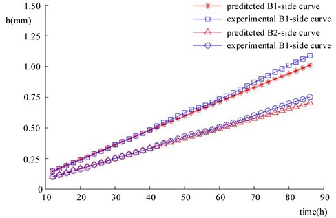
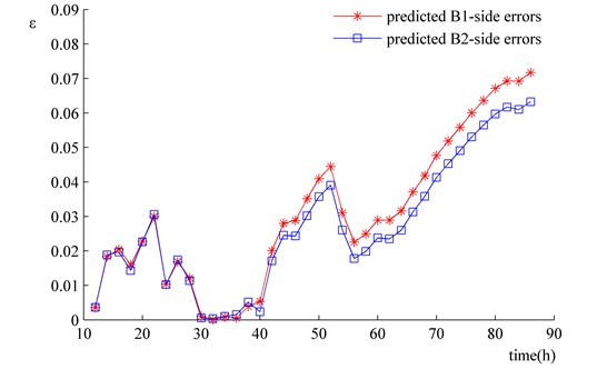
In Fig. 15, the wear predictions of the bushing on Side B1 and Side B2 are on the whole consistent with the experimental results in terms of tendency. However, as the predicted time increases, errors increase accordingly. As shown in Fig. 16, the predicted errors are relatively small within 70 hours, mainly under 5 %. Nevertheless, since the 70th hour, predicted errors gradually grow prominent, which reach the maximum at the 86th hour. Hence, the method developed in the paper is more accurate when it is used to predict small wear loss. Caution must be paid when it is used in large wear loss prediction.

Besides, seeing the unbalanced load effect on the revolute joint, the paper predicts the wear of the revolute joint on both sides. Although the workload is doubled, better prediction results are obtained, which shows that the method proposed by the paper is suitable for the prediction on the working condition of revolute joints under unbalanced load effect.

Fig. 16Predicted errors of the cumulative wear depth of the bushing of Revolute B in the four-bar mechanism

4.5. Analysis of calculative efficiency

In the above simulation prediction, the wear of the bushing from the 12th hour to 86th hour is predicted every two hours. The numerical solution of the mechanism model is operated 38 (= (86 – 10)/2) times, whereas the motion periods of the experimental mechanism from the 12th hour to 86th hour is 43776 (= (86 – 10)×60×9.6). Since the wear of the actual mechanism after 43776 rounds of motion can be predicted with simply 38 times of the mechanism simulations, the method is highly effective and efficient.

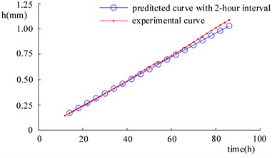
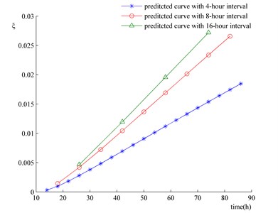
Obviously, if the time interval of 2 hours is extended, the calculative efficiency will be further improved. As shown in Fig. 17, the wear depth changes of the bushing on Side B1 are predicted with time intervals of 4, 8, and 16 hours, respectively, and the data obtained are compared with that acquired in the wear experiment. In Fig. 17, each symbol means one time of mechanism simulation. Hence, the wear predictions with time intervals being 4, 8, and 16 hours need 38, 19, 10 and 5 times of mechanism simulation, respectively. Besides, it can be seen that the curve of the predicted wear coincides that of the wear experiment in terms of their tendency and the relative predicted errors are in the main kept small (see in Fig. 18).

Fig. 19 shows the relative errors between the wear predictions corresponding to time intervals being 4, 8 and 16 hours and those corresponding to time intervals being 2 hours. The longer the time interval is, the larger the relative error becomes. Nonetheless, the relative errors represented by the four curves in Fig. 18 are on the whole small. Therefore, as long as the predicting accuracy is ensured, an appropriately extended time interval helps to promote the computation efficiency of the method, which is of vital significance towards engineering applications.

Fig. 17Comparison of wear prediction results corresponding to different time intervals and experimental results

a)

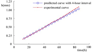
b)

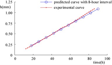
c)

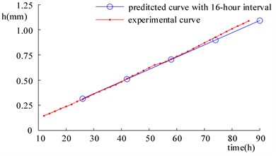
d)

Fig. 18Relative errors between wear prediction results and corresponding to time intervals being 2, 4, 8 and 16 hours and experimental results

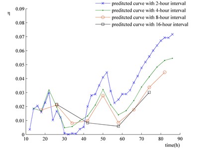
Fig. 19Relative errors between the wear prediction results at time intervals of 4, 8 and 16 hours and those at the time result of 2 hours

5. Conclusions

First of all, the paper proposes a high efficient method for the wear prediction of revolute joint in a planar multi-body system. Second, the method is tried out in the wear prediction of revolute joints with unbalanced loads, and the predictions are verified through experiments. The major conclusions are as follows.

1) When the method is used for wear prediction, it is assumed that the pin and the bushing in a revolute joint are in continuous contact with each other. Hence, the method is applicable solely in mechanisms with low velocity. Besides, it is suggested that the method is used in the wear prediction of revolute joints in the stable wear stage, for it secures the accuracy of prediction results.

2) The method is highly efficient. While the prediction accuracy is ensured, an extended time interval will further promote computation efficiency.

3) The method is highly precise when the clearance wear is relatively small. In circumstances where the clearance wear is large, special attention should be paid to the prediction results as the errors grow large.

4) There exist no ideal planar mechanisms in reality, since their links are always out of plane due to the need of assemblage. This fact results in unbalance loads acted on revolute joints. Hence, for actual engineering mechanisms, the working condition with unbalancing loads is ubiquitous for revolute joints. To predict the wear under such circumstances, application of the method to predict the wear changes on both sides of the revolute joint can provide an insight into the wear evolution of the revolute joint within different time intervals. In this sense, the method proposed by the paper is of high engineering practicability.

References

Bai Z. F., Zhao Y. Dynamic behaviour analysis of planar mechanical systems with clearance in revolute joints using a new hybrid contact force model. International Journal of Mechanical Sciences, Vol. 54, 2012, p. 190-205.

Publisher
Bai Z. F., Zhao Y. Dynamics modeling and quantitative analysis of multibody systems including revolute clearance joint. Precision Engineering, Vol. 36, 2012, p. 554-567.

Publisher
Bai Z. F., Zhao Y., Chen J. Dynamics analysis of planar mechanical system considering revolute clearance joint wear. Tribology International, Vol. 64, 2013, p. 85-95.

Publisher
Rahmanian S., Ghazavi M. R. Bifurcation in planar slider-crank mechanism with revolute clearance joint. Mechanism and Machine Theory, Vol. 91, 2015, p. 86-101.

Publisher
Ma J., Qian L., Chen G., Li M. Dynamic analysis of mechanical systems with planar revolute joints with clearance. Mechanism and Machine Theory, Vol. 94, 2015, p. 148-164.

Publisher
Daniel G. B., Cavalca K. L. Analysis of the dynamics of a slider-crank mechanism with hydrodynamic lubrication in the connecting rod-slider joint clearance. Mechanism and Machine Theory, Vol. 46, 2011, p. 1434-1452.

Publisher
Zheng E., Zhou X. Modeling and simulation of flexible slider-crank mechanism with clearance for a closed high-speed press system. Mechanism and Machine Theory, Vol. 74, 2014, p. 10-30.

Publisher
Erkaya S., Uzmay I. Experimental investigation of joint clearance effects on the dynamics of a slider-crank mechanism. Multibody System Dynamics, Vol. 24, 2010, p. 81-102.

Publisher
Bai Z. F., Zhao Y. A hybrid contact force model of revolute joint with clearance for planar mechanical systems. International Journal of Non-Linear Mechanics, Vol. 48, 2013, p. 15-36.

Publisher
Zhang J., Du X. Time-dependent reliability analysis for function generation mechanisms with random joint clearances. Mechanism and Machine Theory, Vol. 92, 2015, p. 184-199.

Publisher
Pandey M. D., Zhang X. System reliability analysis of the robotic manipulator with random joint clearances. Mechanism and Machine Theory, Vol. 58, 2012, p. 137-152.

Publisher
Wang J., Zhang J., Du X. Hybrid dimension reduction for mechanism reliability analysis with random joint clearances. Mechanism and Machine Theory, Vol. 46, 2011, p. 1396-1410.

Publisher
Dubowsky S., Freudenstein F. Dynamic analysis of mechanical systems with clearances. Part 1. Formulation of dynamic model. Journal of Engineering for Industry, Vol. 93, 1971, p. 305-309.

Publisher
Earles S. W. E., Wu C. L. S. Motion analysis of a rigid link mechanism with clearance at a bearing using Lagrangian mechanics and digital computation. Mechanisms, 1973, p. 83-89.

Search CrossRef
Haines R. S. A theory of contact loss at resolute joints with clearance. Journal Mechanical Engineering Sciences, Vol. 22, 1980, p. 129-136.

Publisher
Erkaya S., Uzmay I. Determining link parameters using genetic algorithm in mechanisms with joint clearance. Mechanism and Machine Theory, Vol. 44, 2009, p. 222-234.

Publisher
Yayli M. A compact analytical method for vibration of micro-sized beams with different boundary conditions. Mechanics of Advanced Materials and Structures, Vol. 24, 2017, p. 496-508.

Publisher
Yayli M. Ö. On the axial vibration of carbon nanotubes with different boundary condition. Micro and Nano Letters, Vol. 9, 2014, p. 807-811.

Publisher
Yayli M. Ö. Free vibration behavior of a gradient elastic beam with varying cross section. Shock and Vibration, Vol. 2014, 2014, p. 801696.

Publisher
Gilardi G., Sharf I. Literature survey of contact dynamics modeling. Mechanism and Machine Theory, Vol. 37, 2002, p. 1213-1239.

Publisher
Pereira M. S., Nikravesh P. E. Impact dynamics of multibody systems with frictional contact using joint coordinates and canonical equations of motion. Nonlinear Dynamics, Vol. 9, 1996, p. 53-71.

Publisher
Thornton C. Coefficient of restitution for collinear collisions of elastic-perfectly plastic spheres. Journal of Applied Mechanics, Vol. 64, 1997, p. 383-386.

Publisher
Ravn P. A continuous analysis method for planar multibody systems with joint clearance. Multibody Systems Dynamics, Vol. 2, 1998, p. 1-24.

Publisher
Lankarani H. M., Nikravesh P. E. A contact force model with hysteresis damping for impact analysis of multibody systems. Journal of Mechanical Design, Vol. 112, 1990, p. 369-376.

Publisher
Tian Q., Zhang Y., Chen L., Flores P. Dynamics of spatial flexible multibody systems with clearance and lubricated spherical joints. Computers and Structures, Vol. 87, 2009, p. 913-929.

Publisher
Ravn P., Shivaswamy S., Alshaer B. J., Lankarani H. M. Joint clearances with lubricated long bearings in multibody mechanical systems. Journal of Mechanical Design, Vol. 122, 2000, p. 484-488.

Publisher
Zukas J. A., Nicholas T., Greszczuk L. B., Curran D. R. Impact Dynamics. John Wiley and Sons, New York, 1982.

Search CrossRef
Machado M., Moreira P., Flores P., Lankarani H. M. Compliant contact force models in multibody dynamics: evolution of the Hertz contact theory. Mechanism and Machine Theory, Vol. 53, 2012, p. 99-121.

Publisher
Reye T. The theory of bearing. Civil Engineer, Vol. 4, 1860, p. 235-255.

Search CrossRef
Archard J. F. Contact and rubbing of flat surfaces. Journal of Applied Physics, Vol. 24, 1953, p. 981-988.

Publisher
Tasora A., Prati E., Silvestri M. Experimental investigation of clearance effects in a revolute joint. Proceedings of the AIMETA International Tribology Conference, Rome, Italy, 2004.

Search CrossRef
Flores P. Modeling and simulation of wear in revolute clearance joints in multibody systems. Mechanism and Machine Theory, Vol. 44, 2009, p. 1211-1222.

Search CrossRef
Mukras S., Kim N. H., Mauntler N. A., Schmitz T. L., Sawyer W. G. Analysis of planar multibody systems with revolute joint wear. Journal of Wear, Vol. 268, 2010, p. 643-652.

Publisher
Mukrasa S., Kima N. H., Sawyera W. G., Jacksonb D. B., Bergquist L. W. Numerical integration schemes and parallel computation for wear prediction using finite element method. Wear, Vol. 266, 2009, p. 822-831.

Publisher
Nikravesh P. E. Computer-Aided Analysis of Mechanical Systems. Prentice-Hall, Englewood Cliffs, NJ, 1988.

Search CrossRef
Baumgarte J. Stabilization of constraints and integrals of motion in dynamical systems. Computer Methods in Applied Mechanics and Engineering, Vol. 1, 1972, p. 1-16.

Publisher
Hunt K. H., Crossley F. R. E. Coefficient of restitution interpreted as damping in vibroimpact. Journal of Applied Mechanics, Vol. 7, 1975, p. 440-445.

Publisher
Khemili I., Romdhane L. Dynamic analysis of a flexible slider-crank mechanism with clearance. European Journal of Mechanics – A/Solids, Vol. 27, 2007, p. 882-898.

Publisher
Shivawamy S. Modeling Contact Forces and Energy Dissipation during Impact in Multibody Mechanical Systems. Wichita State University, Wichita, Kansas, 1997.

Search CrossRef
Schmitz T. L., Action J. E., Ziegert J. C., Sawyer W. G. The difficulty of measuring low friction: uncertainty analysis for friction coefficient measurement. Journal of Tribology, Vol. 127, 2005, p. 673-678.

Publisher
Flores P. Modeling and simulation of wear in revolute clearance joints in multibody systems. Mechanism and Machine Theory, Vol. 44, Issue 6, 2009, p. 1211-1222.

Publisher
Mukras S., Kim N. H., Mauntler N. A., Schmitz T., Sawyer W. G. Comparison between elastic foundation and contact force models in wear analysis of planar multibody system. Journal of Tribology, Vol. 132, 2010, p. 031604.

Publisher
Meng H. C., Ludema K. C. Wear models and predictive equations: their form and content. Wear, Vols. 181-183, 1995, p. 443-457.

Publisher

Cited by

A multibody-dynamics based method for the estimation of wear evolution in the revolute joints of mechanisms that considers link flexibility

(2024)

About this article

Received

16 August 2017

Accepted

18 February 2018

Published

30 September 2018

SUBJECTS

Fault diagnosis based on vibration signal analysis

DOI

https://doi.org/10.21595/jve.2018.18979

Keywords

wear

revolute joint clearance

unbalance loading

multibody systems

Acknowledgements

Support provided by National Natural Science Foundation of China (Grant No. 51305143, 51405168), Promotion Program for Young and Middle-aged Teacher in Science and Technology Research of Huaqiao University (Grant No. ZQN-PY504) and Science and technology planning project of Quanzhou (Grant No. 2017G045) are acknowledged. Authors of the paper gratefully appreciate the helpful suggestions and careful modifications on English expressions of the reviewers.

Author Contributions

Xiongming Lai developed an efficient method to describe the evolution of the revolute joint wear during the process of the mechanism movement, partial experimental design and data analysis and thesis writing. Yisheng Liu designed the test bed, carry out the related experiment and experimental disposal, paper modification. Tianchen Ji designed the test bed, carry out the related experiment and experimental disposal. Cheng Wang took on partial program design, experimental scheme design, and experimental data analysis, paper modification. Yong Zhang took on partial program design, experimental scheme design, and experimental data analysis, paper modification.

This is an open access article distributed under the Creative Commons Attribution License, which permits unrestricted use, distribution, and reproduction in any medium, provided the original work is properly cited.

Previous article in issue Previous Next article in issue Next

Research article

2019 11 28

Dynamic analysis of slider-crank mechanism with clearance fault

Shungen Xiao, Mengmeng Song, Zexiong Zhang

Research article

2018 12 31

An improved extreme-point symmetric mode decomposition method and its application to rolling bearing fault diagnosis

Ping Xia, Hua Xu, Mohan Lei, Zaichao Ma

Research article

2018 09 24

Dynamic analysis of the moving mechanism of the reciprocating compressor with clearance joints

Qingfeng Xiao, Shulin Liu, Ang Nie, Shungen Xiao, Shouguo Cheng

Research article

2018 08 15

Deployment accuracy analysis of cable-strut deployable mechanism with joint clearances and forces constrained

Fei Lin, Jinbao Chen, Chuanzhi Chen, Meng Chen, Zirui Dong, Jinhua Zhou

X. Lai, Y. Liu, T. Ji, C. Wang, and Y. Zhang, “A method for analyzing the revolute joint wear of planar multibody systems and its application in unbalance loading working condition,” Journal of Vibroengineering, Vol. 20, No. 6, pp. 2301–2320, Sep. 2018, https://doi.org/10.21595/jve.2018.18979

Copy Extrica

Copied to clipboard!

TY  - JOUR
DO  - 10.21595/jve.2018.18979
UR  - https://doi.org/10.21595/jve.2018.18979
TI  - A method for analyzing the revolute joint wear of planar multibody systems and its application in unbalance loading working condition
T2  - Journal of Vibroengineering
AU  - Liu, Yisheng
AU  - Lai, Xiongming
AU  - Ji, Tianchen
AU  - Wang, Cheng
AU  - Zhang, Yong
PY  - 2018
DA  - 2018/09/30
PB  - JVE International Ltd.
SP  - 2301-2320
IS  - 6
VL  - 20
SN  - 1392-8716
SN  - 2538-8460
ER  - 

Copy Ris

Copied to clipboard!

@article{Liu_2018,
	doi = {10.21595/jve.2018.18979},
	url = {https://doi.org/10.21595/jve.2018.18979},
	year = 2018,
	month = {sep},
	publisher = {{JVE} International Ltd.},
	volume = {20},
	number = {6},
	pages = {2301--2320},
	author = {Yisheng Liu and Xiongming Lai and Tianchen Ji and Cheng Wang and Yong Zhang},
	title = {A method for analyzing the revolute joint wear of planar multibody systems and its application in unbalance loading working condition},
	journal = {Journal of Vibroengineering}
}

Copy Bibtex

Copied to clipboard!

[1]Y. Liu, X. Lai, T. Ji, C. Wang, and Y. Zhang, “A method for analyzing the revolute joint wear of planar multibody systems and its application in unbalance loading working condition,” Journal of Vibroengineering, vol. 20, no. 6, pp. 2301–2320, Sep. 2018, doi: 10.21595/jve.2018.18979.

Copy IEEE

Copied to clipboard!

Liu, Yisheng, Xiongming Lai, Tianchen Ji, Cheng Wang, and Yong Zhang. “A Method for Analyzing the Revolute Joint Wear of Planar Multibody Systems and Its Application in Unbalance Loading Working Condition.” Journal of Vibroengineering 20, no. 6 (September 30, 2018): 2301–20. https://doi.org/10.21595/jve.2018.18979.

Copy Chicago

Copied to clipboard!

A method for analyzing the revolute joint wear of planar multibody systems and its application in unbalance loading working condition

Abstract

1. Introduction

2. The modeling of multibody dynamic system with clearance

2.1. Multibody dynamic system model

2.2. Clearance model

2.2.1. Description of clearance contact model

2.2.2. Calculation of clearance force

3. A new high efficient method for predicting revolute joint wear

3.1. Calculation of the wear depth of revolute joint

3.2. Calculation of wear depth of revolute joint with wear ranges considered

3.3. The prediction method of revolute joint wear in different motion time intervals

4. Numerical example and experimental validation

4.1. Experimental mechanism introduction

4.2. Analysis of wear range

4.3. The calculation of equivalent wear coefficient

4.4. Wear prediction and verification

4.5. Analysis of calculative efficiency

5. Conclusions

References

Cited by

About this article

Related Articles