A remaining useful life prediction and maintenance decision optimal model based on Gamma process

Pang, Sheng; Jia, Yunxian

Vibroengineering Procedia

Browse Procedia

Published: 08 December 2016

Check for updates

A remaining useful life prediction and maintenance decision optimal model based on Gamma process

Sheng Pang¹

Yunxian Jia²

^{1, 2}Department of Equipment Command and Management, Ordnance Engineering College, Shijiazhuang, China

Corresponding Author:

Sheng Pang

Cite the article Download PDF

Downloads 1383

Abstract

Aiming at the practical problem of maintenance decision-making, the remaining useful life (RUL) prediction method and the maintenance decision optimization model are studied emphatically. Firstly, the condition space model based on Gamma degradation process is established, according to the characteristics of the degradation process of the equipment condition. Then the RUL expectancy is predicted by this model, and the RUL probability density function of the equipment can be got. Finally, this model is validated by the data obtained from the roller bearing life test. The maintenance decision model is established with the minimum cost as the objective, the maintenance decision is optimized, and the RUL prediction and maintenance decision are realized. the example proves the validity and feasibility of this model.

1. Introduction

Some parts of the machinery will be gradually degradated in the course of using, degradation can act as mechanical components wear, crack growth, and corrosion deepening, which is the result of a series of physical and chemical effects. Ultimately result of the equipment degradation is function failure occurs, but the condition of those degradation is often not measurable or difficult to measure directly. In order to obtain the data of the degradation, condition based maintenance (CBM) can be used to extract and analyze the condition data of each device, and indirectly reflect the health condition of each device, so as to the RUL is forecasted, and the maintenance optimization is realized. In this paper, the Gamma degradation process model is used to describe the degradation condition performance [1]. The RUL is measured by the model, and the maintenance decision model is optimized by using the residual life test results.

2. Gamma-SSM degradation model

2.1. Model establishment

Assuming that the degradation of the condition $x$ is in accordance with the Gamma process, $y$ is the observed variable corresponding to $x$ , $x_{i}$ is the condition of equipment at the time of $t_{i}$ , the condition equation and the observed equation of this model are shown in Eq. (1-2) [1]:

1

x_{i} - x_{i - 1} ~ G a m m a (α (t_{i}) - α (t_{i - 1}), λ),

2

y_{i} = Η_{i} (x_{i}) + ε .

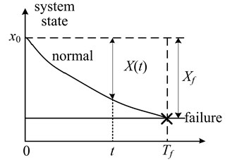
Assuming that the system fails when the $x$ reaches the fault setting $x_{f}$ , as shown in Fig. 1. The time required for the system condition from 0 to the fault is shown in Eq. (3):

3

T_{f} = i n f \{t : x = X_{f}, t > 0\} .

Assuming that the degradation process of the equipment is a stationary Gamma process, and the shape parameter $a (t)$ is a linear function, $a (t) = a \cdot t$ . The relationship between observed quantity $y$ and the condition quantity $x$ is $y = c \cdot x + ε$ , the degradation model can be expressed as Eqs. (4-5) under the condition that the observed sequence is obtained:

4

x_{i + 1} - x_{i} ~ G a m m a (a \cdot (t_{i + 1} - t_{i}), λ),

5

y_{i} = c \cdot x_{i} + ε .

It can be seen from the hypothesis that the $ε$ of observed noise obeys normal distribution with mean 0, that is $y ~ N (c \cdot x, σ)$ . The form of the degradation model can be determined as long as the value of the parameter is obtained.

Fig. 1The degradation process of system

2.2. RUL prediction

The concrete form of the Gamma condition space model can be obtained after determining the parameters of the condition space model, and then the RUL distribution function of the equipment can be got and shown in Eq. (6-8) [2]:

6

F (τ_{i}| y_{0 : c}) = P (τ_{i} + t_{i} \geq T_{f}| y_{0 : i}) = \int p (τ_{i} + t_{i} \geq T_{f}| x_{i}) \cdot p (x_{i}| y_{0 : i}) d x_{i},

7

p (τ_{i} + t_{i} \geq T_{f}| x_{i}) = p (x (τ_{i} + t_{i}) \geq X_{f}| x_{i}) = \frac{Γ (a \cdot τ_{i}, (X_{f} - x_{i}) / λ)}{Γ (a \cdot τ_{i})},

8

p (x_{i}| y_{0 : i}) = f (x_{0 : i} | y_{0 : i}) \approx \sum_{s = 1}^{N_{s}} w_{i}^{s} δ (x_{i} - x_{i}^{s}),

where: $N_{s}$ is the number of partical, $T_{f}$ is the equipment failure time, $w_{i}$ is the weight of the $i$ th, $X_{f}$ is the failure threshold, $y_{0 : c}$ is the observation sequence until the current time, $y_{0 : i}$ is the observation of the current time, is the $i$ th condition monitor time, $x_{i}$ is the condition value of $t_{i}$ time, $x_{1 : i} = \{x_{1}, x_{2}, \dots, x_{n}\}$ is the condition sequence of $i$ th monitor and $y_{0 : i} = \{y_{0}, y_{1}, y_{2}, \dots, y_{n}\}$ is the degradation quantity of $t_{i}$ time.

In addition, the condition probability density function of the prediction time $t_{k}$ can be expressed as Eq. (9):

9

p (x_{k}| y_{0 : i}) = \int p (x_{k}| x_{i}) p (x_{i}| y_{0 : i}) d x_{i} = \sum_{s = 1}^{N_{s}} p (x_{k}| x_{i}^{s}) \cdot w_{i}^{s} .

From the process of particle filter algorithm, the Eq. (8) can be expressed by filtering particles $\{x_{i}^{s}; s = 1,2, \dots, N_{s}\}$ , the RUL distribution function and probability density function can be expressed as Eq. (10-11) [3, 4]:

10

F (τ_{i} | y_{0 : c}) = p (τ_{i} + t_{i} \geq T_{f} | y_{0 : i}) = \int p (τ_{i} + t_{i} \geq T_{f} | x_{i}) p (x_{i} | y_{0 : i}) d x_{i}

\approx \sum_{s = 1}^{N_{s}} p (τ_{i} + t_{i} \geq T_{f}| x_{i}^{s}) \cdot w_{i}^{s} = \sum_{i = 1}^{N_{s}} \frac{Γ (a \cdot τ_{i}, (X_{f} - x_{i}^{s}) / λ)}{Γ (a \cdot τ_{i})} \cdot w_{i}^{s},

11

p (τ_{i}| y_{0 : i}) = \frac{d F (τ_{i}| y_{0 : i})}{d τ_{i}} .

Under the conditions $y_{0 : i}$ , the average RUL can be obtained according to the following Equation:

12

{\bar{T}}_{R U L} = \int_{0}^{+ \infty} (1 - F (τ_{i} | y_{0 : c})) d t .

3. Maintenance decision optimization model

According to the current operating condition of the equipment, the maintenance decision model, which aims at the minimum cost, can be used to determine whether and when the maintenance is to be carried out during the next interval, the failure can be avoided to the greatest extent.

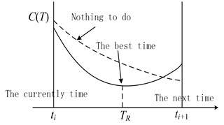
The equipment has two kinds of maintenance strategy: (1) corrective maintenance or failure maintenance, that is the maintenance or replacement activities of the fault product before the scheduled repair time. (2) Preventive maintenance, that is the maintenance or replacement activities when the product reaches its intended repair time [5]. Therefore, the maintenance decision model with minimum cost is established according to the standard of maintenance decision and the residual life probability density function. The decision process is shown in Fig. 2.

Fig. 2The sketch map of maintenance decision-making

3.1. The hypothesis

(1) The condition detection will be completed every $Δ t$ , and the moment data of the current condition will be obtained.

(2) If a fault occurs during the test interval, the repairs can be carried out immediately.

(3) The cost of the preventive maintenance should less than the corrective maintenance, $T_{P} < T_{C}$ .

(4) The initial condition of the equipment will be recovered whether the preventive maintenance or the corrective maintenance.

3.2. The decision model with minimum cost

The cost of equipment components can be expressed as [6]:

13

C (T_{R}) = \frac{E (C)}{E (T)},

14

E (C) = c_{f} \times P_{f} + c_{p} \times P_{p} + n c_{i} = c_{f} \times p (τ_{i} < T_{R} - t_{i} | y_{0 : i}) + c_{p} \times [1 - p (τ_{i} < T_{R} - t_{i} | y_{0 : i})]

+ n \cdot c_{i} = c_{p} + (c_{f} - c_{p}) \cdot p (τ_{i} < T_{R} - t_{i}| y_{0 : i}) + n \cdot c_{i},

15

E (T) = t_{i} + (T_{R} - t_{i} + T_{P}) \cdot [1 - f (τ_{i} < T_{R} - t_{i} | y_{0 : i})] + \int_{0}^{T_{R} - t_{i}} (τ_{i} + T_{c}) f (τ_{i} |y_{0 : i}) d τ_{i})],

16

C (T_{R}) = \frac{c_{p} + (c_{f} - c_{p}) \cdot f (τ_{i} < T_{R} - t_{i}| y_{0 : i}) + n \cdot c_{i}}{t_{i} + (T_{R} - t_{i} + T_{p}) \cdot [1 - f (τ_{i} < T_{R} - t_{i}| y_{0 : i})] + \int_{0}^{T_{R} - t_{i}} (τ_{i} + T_{c}) f (τ_{i} |y_{0 : i}) d τ_{i}},

where: $E (C)$ is the expected total cost for the update cycle, $E (T)$ is the update cycle length, $Δ t$ is the condition monitor intervals time $Δ t = t_{i} - t_{i - 1}; f (τ_{i} |y_{0 : i})$ , $P_{P}$ is the probability of preventative maintenance, $P_{f}$ is the probability of failure maintenance, $c_{p}$ is the costs of preventative maintenance, $c_{f}$ is the costs of failure maintenance, $T_{R}$ is the best time of maintenance replaced, $C (T_{R})$ is the costs during the same time when maintenance replaced time is $T_{R}$ , $t_{i}$ is the condition monitoring points of the current moments $t_{0} = 0$ , $T_{P}$ is the mean time of preventative maintenance, $T_{C}$ is the mean time of corrective maintenance, $c_{i}$ is the costs of each condition monitor and $n c_{i}$ is the total costs of condition monitor.

Since the cost of condition monitor come from equipment, and the sum is relatively small. Therefore, in the actual decision, $n c_{i} = 0$ .

3.3. The best time of maintenance

The maintenance time $T_{R}$ corresponding every monitor time, which possess the minimum maintenance cost, is obtained through the cost decision model. When $T_{R} - t_{i} > Δ t$ , nothing to do, as far as $T_{R} - t_{i} \leq Δ t$ occur, the maintenance or replacement will be carry out. The $T_{R}$ is the best repair time of CBM [7].

4. Application

Three sets of Rexnord ZA-2155 double-row roller bearings were used in test. The full life test of the two sets were completed for model parameter estimation and model verification. The censoring life test of third set is completed for maintenance decision. During the whole life test, the rotational speed is 2000 r/min, and the load is 10000LB (about 44500 N). The frequency is 20 kHz and the length is 1 s. there is a strong noise occur in 966 h and 982 h of bearing 1 and bearing 2 respectively. The indirect condition observation data $y$ is the average energy of the vibration signal, the condition data $x$ is the the wear amount. The average energy chang is shown in Fig. 3.

The model parameters are estimated by using the indirect condition observation data of bearing 1, and the parameters of RUL are calculated. [8] The date is shown in Table 1. The condition space model based on the Gamma degradation process can be obtained by the model parameters, the probability density function of the bearing RUL $f (τ_{i} |y_{0 : i})$ can be obtained by the above equations.

Table 1Model parameter calculation result

Parameters	$a$	$λ$	$c$	$σ$
Mean value	0.3542	153.2	7563	1869

The RUL prediction method is realized by MATLAB 7.0. using the observation data of bearing 2, the probability density function of RUL at different condition monitor time (500 hours to 750 hours) is shown in Fig. 4. The real values and the estimated values of the RUL at different detection time are shown in Table 2.

Fig. 3The average energy change of two sets bearing

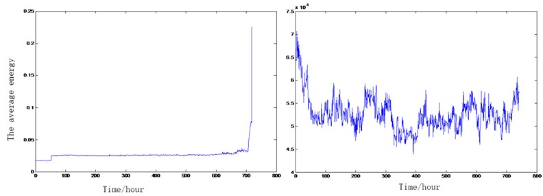
Fig. 4RUL probability density at different time (where: * denotes the estimated value of the RUL, △ representing the true value of the RUL)

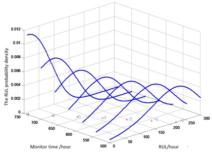
Table 2True value and estimated value of residual life

Monitor time	500	540	580	620	660	700	740
True value	241	201	161	121	81	41	1
Forecast values	220	184	148	112	75	39	2

The maintenance decision of the best maintenance time is completed using the date of bearing 3. Assuming $c_{p} =$ 600, $c_{f} =$ 1200, brought $f (τ_{i} |y_{0 : i})$ into Eq. (16) after taking the probability density function of the RUL. The optimal replacement time $T_{R}$ with minimum cost of every monitor are obtained, and shown in Fig. 5.

Fig. 5The optimal replacement time at different monitor

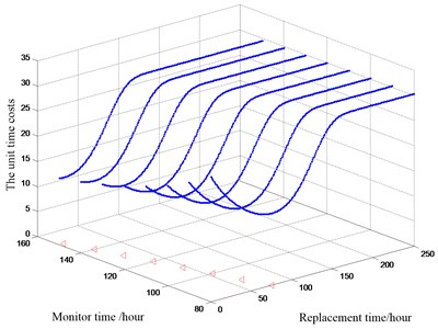
As we can see in the Fig. 5, the unit time costs decrease first and then increases, as the replacement time increases. the optimal maintenance time can be obtained at the extreme point. △ representing the replacement time with lowest per unit time at each monitor time. When the condition $T_{R} - t_{i} \leq Δ t$ is satisfied for the first time, $T_{R} =$ 156 h can be calculated by Matlab. So, when the replacement time is 156 hours, the unit time cost trend to minimum $C (T_{R}) =$ 1306.

5. Conclusions

By studying the failure mechanism of the product, the condition spare model is established based on Gamma process, the distribution function and probability density function of RUL (RUL) are obtained by this model. The maintenance decision model with the most proper replacement time and the minimum cost is founded up. It can be seen from the above results that the model has some practicality for bearing RUL prediction under the background of this kind of test, and the result shows that the model is practical and effective.

References

Noortwijk J. M. V. A survey of the application of Gamma processes in maintenance. Reliability Engineering and System Safety, Vol. 94, 2009, p. 2-21.

Search CrossRef
Sikorska J., Hodkiewicz M., Ma L. Prognostic modelling options for remaining useful life estimation by industry. Mechanical Systems and Signal Processing, Vol. 25, 2011, p. 1803-1826.

Search CrossRef
Park J. I., Bae S. J. Direct prediction methods on lifetime distribution of organic light-emitting diodes from accelerated degradation tests. IEEE Transactions, Vol. 59, 2010, p. 74-90.

Search CrossRef
Polson N. G., Stroud J. R., Muller P. Particle Filtering with Sequential Parameter Learning. University of Pennsylvania Working Paper, 2006, p. 47-49.

Search CrossRef
Gan Mo-zhi, Kang Jian-she, Gao Qi Military Equipment Maintenance Engineering. National Defense Industry Press, Beijing, 2005, p. 1-3.

Search CrossRef
Jia Xi-sheng The Decision Models for Reliability Centered Maintenance. National Defense Industry Press, Beijing, 2007, p. 71-86.

Search CrossRef
Argon C., Wu G. S. Real-time health prognosis and dynamic preventive maintenance policy for equipment under aging Markovian deterioration. International Journal of Production Research, Vol. 45, 2007, p. 3351-3379.

Search CrossRef
Si Xiao-Sheng, Wang Wen-Bin, Hu Chang-Hua RUL Estimating – a review on the statistical data driven approaches. European Journal of Operational Research, Vol. 213, 2011, p. 1-14.

Search CrossRef

About this article

Received

02 November 2016

Accepted

03 November 2016

Published

08 December 2016

SUBJECTS

Fault diagnosis based on vibration signal analysis

Keywords

maintenance decision

remaining useful life (RUL)

Gamma process

cost optimization

This is an open access article distributed under the Creative Commons Attribution License, which permits unrestricted use, distribution, and reproduction in any medium, provided the original work is properly cited.