A remaining useful life prediction method for engineering components based on intelligent product limit estimator

2.1. Kaplan-Meier nonparametric estimation

Kaplan-Meier nonparametric estimation is one type of product limit estimation. This method should be used to find out that both the life data and the right deleted data are known exactly, that is, it cannot be interval data. By observing the lifespan of n individuals of population $T$, we can get $t_1,t_2,\dots t_n$ (there may be right-censored data, but no left-censored data). When $t_i$ is terminal data, let ${\delta }_i=1$; When $t_i$ is right-censored data, let ${\delta }_i=0$, our data can be recorded as $\left(t_i,{\delta }_i\right)$, $i=\mathrm{1,2},\dots ,n$.

Rearrange these $t_i$ from small to large, when a deleted data is equal to a final data, then the end of life data is placed before the deleted data $t_{\left(1\right)}\le t_{\left(2\right)}\le ...\le t_{\left(n\right)}$.

When $t_{\left(i\right)}$ is the end of life data, mark ${\delta }_{\left(i\right)}=1$; When $t_{\left(i\right)}$ is right-censored data, mark ${\delta }_{\left(i\right)}=0$$\left(1\le i\le n\right)$.

The product limit of $S\left(t\right)$ is defined as follows:

When $t<t_n$, $\widehat{S}\left(t\right)$ has the following unified expression:

Here, it is agreed that $\prod _{\varnothing }{a}_i=1$ and $\varnothing$ is an empty set.

2.2. Time series prediction based on parallel multilayer perceptron and residual fitting

Because of the irregularity of chaotic time series, the key part of neural network prediction is to learn the law of data, and then get the network that can best express the law characteristics of data series. The parallel multi-layer perceptron (PMLP) network composed of multiple parallel MLPs is used to predict chaotic time series, which can improve the prediction accuracy and network performance. Here, each MLP has a different number of input nodes, and then the combination weight coefficient of the parallel MLP network is determined by the least square method, for the sake of obtaining the best combination of the number of input nodes.

3.1. Data acquisition

The performance of the proposed method is verified through the remaining useful life prediction of spindle bearing from the water pump. The bearing type is deep groove ball bearing SKF 6209. The specific parameters of the bearing are: inside diameter 45 mm, outer diameter 85 mm, and thickness 19 mm. The data of the rolling bearing were acquired from a simulation test bed. The horizontal vibration signals of the bearing were collected by the horizontal acceleration sensor with the 2 min recording interval and 25.6 kHz sampling frequency. 40 sets of vibration data were collected, among which 30 sets of truncated data are used as training samples while the remaining 10 full life data samples are used as test samples.

3.2. Test results

The verification of the proposed method including three steps: constructing the PMLP network, construction of the survival state parameter table collection, and prediction of residual service life of key components. The detailed steps are illustrated as follows.

Step 1: Performance degradation index sequence prediction based on PMLP network prediction and residual fitting.

Training the PMLP network with the training samples until the specified accuracy is reached. The PMLP network is composed of three subnetworks. The number of hidden layer nodes in MLP network is determined by the empirical formula $a=\sqrt{n_1+n_2}+k(0\le k\le 10)$. Tansig function and purelin function are utilized in the hidden layer and the output layer respectively. The maximum training time is set to 1500. The gradient descent method with momentum and adaptive learning rate is adopted for network training. The optimal weight allocation of the three subnetworks is $\omega =\left[0.5980\mathrm{}\mathrm{}0.402\right]$. Then, the data samples are predicted to obtain the degradation index sequence, whose definition is: residual = the true value of the index – the predicted value of the network. The prediction results of PMLP network is adjusted according to the predicted residual, which is fitted with 4th order polynomial. Fig. 1 shows the predicted results and residual results of the index sequence.

Fig. 1The predicted results and residual results of PMLP network

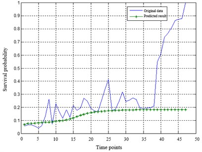
a) The predicted results by the PMLP network

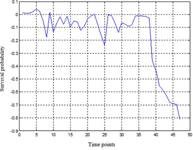
b) The residual results by the PMLP network

Based on the residual error fitting function, the function values of the variables can be obtained and the residuals sequence is extended. Then, the obtained iterative predicted value of degradation index is corrected with the formula “The final predicted value = PMLP network prediction - fitting residual error”.

According to the fitting function of the residual, the residual value of the subsequent points can be obtained by inputting several data values before the truncation point into the trained PMLP neural network for iterative prediction. And then the QE predicted value after the truncation point can be obtained. Finally, the extrapolated residual value was added to the predicted value of QE to correct the predicted value of QE.

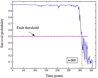
The sample data after the truncated points were added and improved, so as to directly obtain the bearing performance degradation characterization parameter set within the whole life cycle. When the health indicator (CV value) is less than a certain threshold, the device is in critical condition. Therefore, when the index is higher than the threshold value of 0.5, the equipment is deemed to have failed. For the truncated data samples after completion, the data points exceeding the settled failure threshold need to be discarded, that is, the truncated data samples after preprocessing need to be fine-tuned.

Step 2: Construction of the survival state parameter table collection based on the product limit estimation.

20 out of the 30 training samples are pretreated by using the above method, namely the degradation index samples of truncated data are supplemented into complete data samples. While the remaining 10 groups of bearing data samples are still truncated data without preprocessing. Based on the intelligent product limit estimation method, the survival state parameter list collections were constructed for the two types of data as follows.

1) The construction method of preprocessed samples.

Find the failed time interval of the samples. For the training samples earlier than the failed time interval, the survival probabilities of them are set to 1. The survival probabilities of the remaining samples are set to 0.

2) The construction method of truncated samples.

The number of failed bearing samples and the number of withdrawn samples in each time interval was counted among the 30 sample sets. The survival probabilities of 10 truncated samples in each time interval are calculated with the K-M estimation rule.

Step 3: Prediction of residual service life of key components based on feedforward neural network.

The residual service life of the bear is predicted based on the feedforward neural network that consists of three layers. The input layer of the network contains seven nodes. The input vectors are respectively the degradation index QE value of T bearing at the current moment and the degradation index value of the previous six moments. The outputs are the survival probability values in the 5 time periods after the current time period. The FFNN network is trained with the back propagation (BP) algorithm. The survival probability curve of any test sample can be drawn in units of time point and time period respectively after predicting with the constructed neural network, as shown in Fig. 2.

Fig. 2The survival probability prediction of a test sample in units of time point and time interval

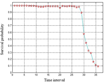
The survival probabilities of the 10 bearing test samples are predicted with the intelligent product estimator and listed in Table 1. It can be seen that the relative error between the predicted value and the true value is less than 10 %. To achieve accurate residual life prediction, the halfway point of the bearing in a time interval is regarded as the end points in whole life cycle in this example. Namely when the survival probability prediction result is the $k$-th time interval, the failure time of the test example is $(k\times 10+k\times 9)/2=9.5k$. The confidence interval for failure time prediction is [9k, 10k], and the confidence is larger than 90 %. In summary, the prediction accuracy of typical bearing residual service life based on the intelligent product limit estimator method is higher than 85 % and the confidence is higher than 90 %.