Abstract
Rolling bearing reliability assessment and remaining useful life (RUL) prediction are crucially important for improving the reliability of mechanical equipment, reducing the probability of sudden failure, and saving on maintenance costs. Novel prediction method is proposed based on PCA and Improved Logistic Regression Model (ILRM) to solve the problem that the model is difficult to establish and the remaining life of rolling bearing is difficult to estimate. Time domain, frequency domain, and time-frequency domain feature extraction methods are employed in this study to extract the original features from the vibration signals. Next, the relative feature value is used to reduce the influence of random vibration and individual differences between bearings. PCA is run based on the original extracted features and high dimensional and superfluous information to merge the original features and reduce the dimension, where typically sensitive features are extracted. The ILRM is then used to build a model that reflects the deterioration trend and eliminates the impact of fluctuations, ultimately yielding information regarding the rolling bearing’s reliability and the remaining life. The proposed method is shown to accurately predict the lifespan of rolling bearings, thus exhibiting practical value in the engineering field.
1. Introduction
Rolling element bearings are a common component in rotating machinery. They can be dangerous, as fault occurring in the bearings may lead to equipment failure [1]. About 30 % of all types of fault in rotating machinery are caused by the fault of rolling bearings [2]. To this effect, accurately predicting the residual life of bearings is important to implement in condition-based maintenance and ultimately prevent unexpected failures. Jardine et al. [3] found that bearing life prediction methodologies fall into three main categories: Statistical approaches, artificial intelligence (AI) approaches, and model-based approaches. Heng et al. [4] proposed two models for predicting rotating machinery failure: Physics-based prognostics and data-driven prognostics models. Each method has its own advantages and disadvantages. At present, the AI and data-driven models are the most popular for RUL prediction. The traditional approach is mainly used in demographic, economic, and medicinal fields, but it is not sufficient for predicting the life expectancy of industrial components such as rolling bearings [5]. Ding [6] used a proportional hazards model to determine the reliability of railway locomotive wheel bearings based on the equipment vibration signal of the kurtosis value, square root value, and other factors. Zhang [7] studied the predictive RUL of a high-pressure water pump bearing based on the Weibull proportional hazard model. Jaouher [8] studied on the bearing life prediction of Weibull and artificial neural network based on the data-driven method. Caesarendra [9] combined the relevance vector machine and logistical regression for machine degradation assessment, and Tran [10] combined the proportional hazard model and support vector machine for machine performance degradation assessment and RUL prediction. Lin and Tseng [11] combined Weibull PHM and vibration-based machine condition monitoring techniques to estimate several machine reliability statistics. However, these methods all require specific mechanical knowledge, and require that many assumptions be made regarding the model parameters and probability density function.
PCA can be used to reduce the feature space dimension, while the principal component subspace offers high to low dimensional data in mean square error data compression, which can minimize variance. In practical applications, multiple features are often required to describe the bearing characteristics. In this study, 15 characteristic parameters were chosen to characterize the bearing degradation process. Excessive information redundancy affects the modeling accuracy, so the main characteristic of focus is dimension reduction. The traditional correlation coefficient method can reduce the dimension, but some useful information is lost in the process. PCA integrates an array of characteristics to achieve dimension reduction without loss of information. Sun et al. [12], for example, successfully used PCA for rotating machinery fault diagnosis. This paper, similarly, proposes a PCA-based dimension reduction method through which important information is retained in predicting the residual life of industrial bearings.
The variable relationship between objects is the primary focus of most research on logistic regression modeling [13]. The biggest difference between logistic and linear regression is that the variable is a mutable variable. For example, the health status of mechanical equipment is divided into normal, early failure, medium-term failure, and serious damage. Because the model has few parameters and is easy to estimate, likelihood estimation methods are applicable to parameter estimation. Said parameters are easily estimated and do not need to be assumed compared to the Weibull proportional hazards model [14]. The independent variables are discrete, continuous, or dummy variables. Characterization of device performance from normal to failure requires an effective understanding of multiple characteristics, logistics analysis results, and equipment descriptions in the multiple characteristics. This is highly desired information for equipment engineers in regards to developing maintenance plans. Yan and Lee [15] proposed a real-time performance model of an elevator door through online data input to a logistics regression model; Chen [16] proposed a tool reliability evaluation method based on the logistics model with vibration signals as inputs. The logistics regression model is not without limitations. In the process of reliability function calculation, accounting solely for current characteristics means the model fails to reflect deterioration trends in bearing vibration signal characteristics. In this study, we improved the logistics regression model to create the proposed ILRM to overcome the shortage of logistics regression model.
This paper provides an approach that combines PCA and ILRM based on relative multivariable to predict the residual life of rolling bearings. Hard failure and multiple degradation features are taken into account. Due to individual differences between bearings, some interference occurs in residual life prediction; the proposed method contains relative features which compensate for this. Relative features are not affected by individual differences among bearings and can be easily calculated. They are well-suited as RUL index for these reasons. The first and second principal components, which can accurately reflect the performance degradation process through PCA, are selected as the covariates of ILRM to predict the RUL. We ran experiments to validate the model that showed it not only enhances the prediction accuracy of previous similar models, but is readily applicable to multiple types of bearings.
2. Theoretical background
2.1. PCA
For a given feature vector set , the -dimensional vector is extracted from the vibration signal of the rolling bearing. The state of machinery can be described by the vector , the covariance matrix of which is expressed as follows:
where represents the number of training samples and represents average value, expressed as:
The eigenvalues (1, 2,…, ) and eigenvectors are obtained from . Then the eigenvalues are arranged in order from large to small: the corresponding feature vector is (1, 2,…, ). The sample projects onto the feature vector to get the principal component in the direction [17]:
All feature vectors form an n-dimensional orthogonal space. The n-dimensional principal component could be obtained from the n-dimensional space onto which is projected. The contribution of the feature rate vector is proportional to its eigenvalues after reconfiguration. The cumulative contribution rate of the firstprincipal component of orthogonal space is expressed as follows:
should be arranged in order from small to large and the contribution rate should be selected as necessary. 95 % means the first principal components consist of 95 % original data. The first principal components can thus be taken to represent the original information, which ensures it is not lost after realizing dimensional reduction.
2.2. Logistics regression model and ILRM
The bearing state is represented by a series of characteristic parameters. The logistics regression model evaluates the bearing state when the data sample is composed of characteristic parameters and the bearing state [18]. The vector can represents the covariate variables which affect the state parameters of the bearing, where represents the number of covariate variables. The conditional probability of the event that does not occur () is expressed as follows:
where , ,…, are the regression coefficients of the covariate variable and .
The bearing state is divided into normal and failure states at . The normal state is replaced by the failure state is replaced by The covariate variable represents the characteristic signal parameters from the state of machinery at the point in question. There is a nonlinear relationship between the state of rolling bearing and covariate variable .
The covariate variable of rolling bearing is . The ratio of bearing reliability function to accumulation failure distribution function is expressed as follows:
The parameters can be solved by the maximum likelihood estimation method, the logarithmic form of which is expressed as follows:
The intercept is a constant term, , ,…, are the weights of covariate variables, means indicates that the event occurrence probability increases as characteristic parameter , increases; means the independent variable has no influence on this model. The logistics model is nonlinear, so , ,…, can be estimated via maximum likelihood estimation method using to denote the maximum likelihood estimate of . The bearing reliability function is:
The logistics regression model ignores the former degradation trend and cannot adapt to fluctuation, which weakens the precision of the residual life prediction model. This paper proposes the ILRM, in which the degradation trend of the rolling bearing is considered during residual life prediction without being subject to fluctuations. The reliability function of the ILRM is expressed as follows:
where is the function of . The function can be used to express the characteristic parameters that reflect the state of the rolling bearing.
The related functions of the ILRM are as follows:
where () is related to the difference between the eigenvalues at and the eigenvalues at moment. is the product of and the corresponding covariates . is the mean values of in a normal work period.
Eqs. (11-12) reflect the fact that the ILRM not only considers the influence of the bearing’s deterioration tendency and reduces the influence of random fluctuations, but also that the amplitude and characteristic trends are almost unchanged compared to the original data. Eq. (10) suggests that the ILRM is not only unaffected by the manufacturing and installation of the individual bearings, but also has a strong generality and accuracy.
The logarithmic form of the likelihood function is expressed as follows:
If covariate variable is predicted, the rolling bearing residual life at moment cays approximately expressed as [19]:
The logistics regression model only considers the bearing characteristic parameters and ignores the bearing degradation trend, so it is susceptible to interference. The result of residual life prediction adds error to the reliability assessment. The ILRM, conversely, considers the bearing degradation trend and decreases the effect of random signal fluctuations, so it yields more accurate prediction results.
3. Methodology
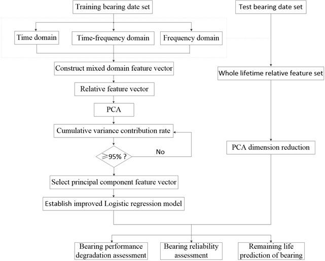
The proposed method was designed to reduce the data fluctuation influence on the RUL, to encompass the degradation features of the bearing, and to achieve highly accurate bearing RUL prediction. A flow chart of the proposed method is shown in Fig. 1.
Fig. 1The flow chart of the proposed method
The individual steps to the proposed method can be described as follows.
1) Select effective feature parameters from the time, frequency, and time-frequency domains.
2) Establish the relative feature vectors of training samples.
3) Carry out PCA and select the principal component vector with the cumulative contribution rate of more than 95 %.
4) Build the ILRM and estimate the model parameters according to the selected principal component vectors.
5) Set up the lifecycle feature set of the test samples; select the relative feature vectors after PCA dimension reduction.
6) Take the selected relative vectors of the testing bearing as the ILRM covariates to complete the performance degradation assessment, reliability assessment, and remaining life prediction of the bearing.
4. Experimental analysis and application
The total life cycle accelerated bearing performance and degradation test data for the rolling bearings used in this paper were provided by the Center for Intelligent Maintenance Systems (IMS), University of Cincinnati [20]. Four tests were conducted on the bearing test rig. A Rexford ZA-2115 was stalled on one shaft as shown in Fig. 2; the bearings contained 16 rollers in each row with a pitch diameter of 2.815 in, roller diameter of 0.331 in, and tapered contact angle of 15.17°.
The rotational speed of the rolling bearing was kept constant at 2000 rpm. A radial load of 6000 lbs was added to the shaft and bearing by a spring mechanism. The vibration signals were collected on a National Instruments DAQ Card 6062E every 20 min through eight high-sensitivity quartz ICP accelerometers installed at vertical and horizontal directions.
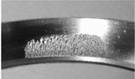
The test was conducted over 35 days at which point a significant amount of metal debris was found on the magnetic plug of the test bearing. This process made it possible to build bearing run-to-failure data sets with known defects. Each data set describes a run-to-failure experiment in which the data sampling rate is 20 KHz and the data length is 20480 points. Three tests (denoted 1, 2, and 3, each containing four bearings) were run to comprise the experiment. Bearing1 of test 2, bearing 3 of test 1, bearing 4 of test 1, and bearing 3 of test 3 were the only components that failed during the experiment. The test results are described in Table 1; Fig. 3 shows the components of the failure bearing.
Fig. 2Bearing test rig and sensor placement illustration
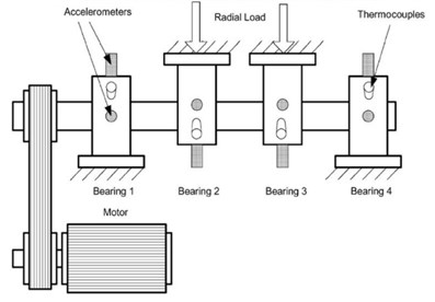
Table 1Tested bearings information
Test# | 1 | 2 | 3 |
Failed bearing | B3, B4 | B1 | B3 |
Failure modes | B3(i), B4(r&o) | B1(o) | B3(o) |
Censored bearing | B1, B2 | B2, B3, B4 | B1, B2, B4 |
Fig. 3Components of failure bearing
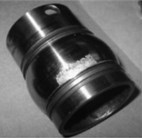
a) Inner race defect
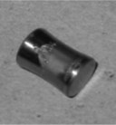
b) Roller element defect
c) Outer race defect
4.1. Feature set selection and processing
Eighty-two feature parameters of time, frequency and time-frequency domain were extracted from the life cycle data of 11 groups of bearings. To reduce the amount of computation and to reduce the PCA dimensions at the same contribution rate, features that did not reflect the bearing state were discarded. Fifteen effective features were selected from the characteristic curve of 82 parameters. The selected features effectively reflect the bearing degradation process, as shown in Fig. 5.
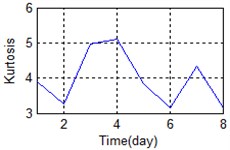
Time domain: Kurtosis, Peak to peak, IMF1 energy spectrum, IMF2 energy spectrum, Variance, Average power, Absolute mean value (AMV), Standard deviation, Pulse factor, Clearance factor, and Kurtosis Factor.
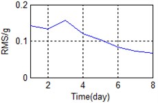
Frequency domain: RMS, and Peak value.
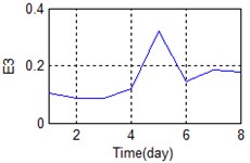
Time-frequency domain: The 3rd frequency bands normalized energy spectrum (E3), and the 7th frequency bands normalized energy spectrum (E7) [21].
Errors in the installation of sensors or in the manufacturing may have caused substantial differences between the measured signals. The means of some features in time, frequency, and time-frequency domain are shown in Fig. 4 for the sake of comparison.
Fig. 4The comparison of feature parameters
a) Time-frequency domain – E3
b) Time domain – Kurtosis
c) Frequency domain – RMS
The same parameters may vastly differ among different bearings. The original data interferes with subsequent data analysis steps and RUL prediction results. In order to overcome the shortage, so relative features can be put out to mitigate this:
where is the relative feature, is the original feature, and is the mean value of the normal period.
A stable trend occurs in the normal period which can be selected to obtain mean values. The relative feature of the rolling bearing can then be acquired by calculating the ratio between the actual value and the mean value. The results are shown in Fig. 5.
4.2. PCA dimension reduction processing
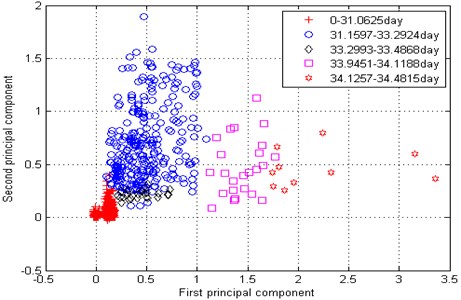
Fig. 5 shows the feature parameters that reflect bearing degradation trends. The parameters reflected by the state of the rolling bearing are not uniform. As mentioned above, it is difficult to determine which parameters reflect the bearing degradation trend; this makes any method of extracting a useful and comprehensive bearing feature particularly important. Here, we use PCA dimension reduction processing to secure the above objectives. The results are shown in Table 2. The contribution rate of the second principal component reached 96.57 %, exceeded the target of 95 %, so the top two principal components were utilized for subsequent analysis here.
Our projection of the first two principal components obtained into two-dimensional space is shown in Fig. 6 and Table 3. Fig. 6 shows that the first principal component reflects the deterioration trend of the bearing. Normal period, early fault, medium wear stage, and severe wear stage occurred in the first principal component. The early failure stage is more prominent in the second principal component because small spalling or cracks are formed in the early failure stage. A healing stage occurs between the early failure and medium wear stage, because in this stage, the surface is smoothed by continuous rolling contact.
Fig. 5Relative characteristics of whole lifetime

a) Time-frequency domain – E3

b) Time-frequency domain – E7

c) Frequency domain – RMS

d) Frequency domain – Peak

e) Time domain – Kurtosis

f) Time domain – Peak to peak

g) Time domain – IMF1

h) Time domain – IMF2

i) Time domain – Avarage power

j) Time domain – Variance

k) Time domain – AMV
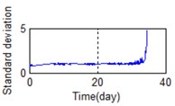
l) Time domain – Standard deviator
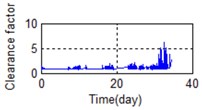
m) Time domain – Clearance factor
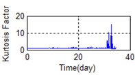
n) Time domain – Kurtosis Factor
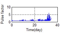
o) Time domain – Pulse factor
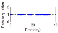
p) Data acquisition time distribution
Table 2The result of PCA
Contribution rate | First principal component | Second principal component | Third principal component |
Relative feature set | 91.17 % | 96.57 % | 97.81 % |
Actual feature set | 86.67 % | 89.53 % | 93.69% |
Table 3The messages of points
Period | Point | Date (day) |
Normal working stage | Red + | 0-32.0625 |
Early failure stage | Blue ○ | 31.1597-33.2924 |
Healing stage | Black ◇ | 33.2993-33.4868 |
Wear medium stage | Magenta □ | 33.9451-34.1188 |
Severe wear stage | Red ☆ | 34.1257-34.4815 |
In conclusion, the top two principal components identified here do accurately express the performance degradation trend of industrial bearings. They not only contain most of the bearing degradation state information, but also greatly reduce the feature dimension. We thus selected the top two principle components as the covariates of the ILRM to predict the RUL in our subsequent assessment.
Fig. 6The top two principal components
4.3. Residual life prediction
In order to verify the effectiveness of the proposed algorithm, we used the logistics regression model to compare the results against the proposed algorithm. The maximum likelihood estimation method was used to estimate the parameters of the logistics regression model and ILRM according to Eq. (7) and Eq. (13). The results are shown in Table 4.
Table 4Model parameters of ILRM and Logistics Regression Model
Model | |||
Improved logistic regression model | 5.358 | 1.742 | 9.458 |
Logistic regression model | 3.187 | 6.528 | 15.734 |
The first and second principal components of the large dimension were introduced into the ILRM and logistics regression model as covariates to represent the reliability of the whole life of bearings, as shown in Figs. 7-8.
Fig. 7 shows that the ILRM tends to decrease along the progression of time during the normal period, which is consistent with the actual situation. The reliability curve of the logistic regression model showed no downward trend under normal conditions (Fig. 8). Fluctuations in the ILRM curve were significantly reduced compared to the logistic regression curve during the normal period.
Fig. 7Reliability curve of improved logistics regression model
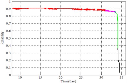
Fig. 8Reliability curve of logistics regression model
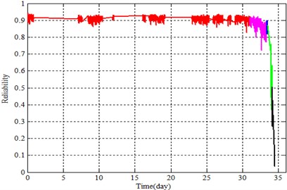
According to Williams [22], a bearing in the wake of the early fault has a healing period. In this period, bearing characteristic values decrease while reliability seems to increase, but actually decreases. This is mainly because early fault cracks are worn down. There is a rising trend in the healing stage as shown in Fig. 8, which introduces interference to the maintenance plan. The algorithm proposed in this paper mitigates this problem as it is shown in Fig. 7. This is mainly due to the logistics regression model, which does not account for the deterioration trend of the bearing prior to analysis.
Table 5 shows the RUL estimated by the ILRM and logistics regression model.
Table 5RUL of bearings in ILRM and logistics regression model
Bearing condition | Normal working stage | Early failure stage | Healing stage | Wearing medium stage | Sever wear stage |
Time (day) | 30.5 | 32.6 | 33.3 | 34 | 34.2 |
Actual RUL | 3.9815 | 1.8815 | 1.1815 | 0.4815 | 0.2815 |
Logistics regression model | 8.3542 | 3.52 | 2.9491 | 1.2201 | 0.8371 |
Estimation error | 4.3727 | 1.6385 | 1.7676 | 0.7386 | 0.5556 |
Improved logistics regression model | 6.3841 | 3.2147 | 2.0031 | 1.0296 | 0.3146 |
Estimation error | 2.4026 | 1.3332 | 0.8216 | 0.1905 | 0.0331 |
The prediction accuracy of the ILRM is much higher than that of the logistics regression model, as shown in Table 5. Take the severe wear stage for example: At 34.2 days, the actual RUL is 0.2815 days; the RUL predicted via ILRM is 0.3146 days while that predicted by the logistics regression model is 0.8371 days. The accuracies were evaluated as follows:
The accuracy of ILRM is 89.48 % while that of the logistics regression model is 33.63 %. The ILRM prediction results are consistent with the residual life of the actual bearing, but the logistics regression model prediction results are volatile and with larger margin of error. This is because the logistics regression model only considers the characteristic of the current time, ignores the degradation trend, and fails to adapt to the fluctuations; the ILRM mitigates these disadvantages.
5. Conclusions
The ILRM was developed in this study in order to resolve problems inherent to the logistics regression model. The proposed model takes into account bearing deterioration trends and adapts to fluctuations in the bearing by increasing and optimizing the covariate selection process. Covariates are selected based on relevant time, frequency, and time-frequency domain features. The method calls for the top two principal components which can accurately describe the performance degradation process of the bearing to be selected experimentally as the ILRM covariates. The proposed method has the following advantages:
1) Based on the relative multi-features, the principle components include sufficient information about the status of bearings to avoid the limitations of traditional kurtosis value, RMS value, and other insufficient factors. Using the principle components as the ILRM covariates allows the reliable and accurate prediction of bearing RUL.
2) The relevant features in the proposed method also reduce the influence of installation, manufacturing, and working conditions; the ILRM has strong generality.
3) The ILRM solves problems that the logistics regression model cannot, specifically in regards to the degradation trend and ability to adapt to bearing fluctuations. It not only yields highly accurate remaining life prediction results and eliminates the impact of fluctuations, but also eliminates the influence of the healing stage, which makes it suited to assisting in timely maintenance decisions.
References
-
Hong B. Vibration Monitoring and Diagnosis of Rolling Bearings – Theory, Method, System. China Machine Press, Beijing, 1996.
-
Sheng Z., Yin Q. Technology and Application of Equipment Condition Monitoring and Fault Diagnosis. Chemical Industry Press, Beijing, 2003.
-
Jardine A. K. S., Line D., Banjevic D. A review on machinery diagnostics and implementing condition-based maintenance. Mechanical Systems and Signal Processing, Vol. 20, 2006, p. 1483-1510.
-
Heng A., Zhang S., Tan A. C. C., Mathew J. Rotating machinery prognostics: state of the art, challenges and opportunities. Mechanical Systems and Signal Processing, Vol. 23, 2009, p. 724-739.
-
O’Connor P. D. T. Commentary: reliability-past, present, and future. IEEE Transactions on Reliability, Vol. 54, Issue 1, 2005, p. 3-10.
-
Ding F., He Z. Reliability evaluation of proportional failure rate model based on equipment state vibration characteristics. Journal of Mechanical Engineering, Vol. 45, Issue 12, 2009, p. 89-94.
-
Zhang Q., Cheng H., Xu G. A mixture Weibull proportional hazard model for mechanical system failure prediction utilizing lifetime and monitoring data. Mechanical Systems and Signal Processing, Vol. 43, 2014, p. 103-112.
-
Jaouher B., Brigitte C., Lotfi S., et al. Accurate bearing remaining useful life prediction based on Weibull distribution and artificial neural network. Mechanical Systems and Signal Processing, Vols. 56-57, 2015, p. 150-172.
-
Caesarendra W., Widodo A., Yang B. Application of relevance vector machine and logistic regression for machine degradation assessment. Mechanical Systems and Signal Processing, Vol. 24, 2010, p. 1161-1171.
-
Tran V., Pham H. Machine performance degradation assessment and remaining useful life prediction using proportional hazard model and support vector machine. Mechanical Systems and Signal Processing, Vol. 32, 2012, p. 320-330.
-
Lin C. C., Tseng H. Y. A neural network application for reliability modelling and condition-based predictive maintenance. International Journal of Advanced Manufacturing Technology, Vol. 25, 2005, p. 174-179.
-
Sun W., Chen J., Li J. Decision tree and PCA-based fault diagnosis of rotating machinery. Mechanical Systems and Signal Processing, Vol. 21, Issue 3, 2007, p. 1300-1317.
-
He X. Practical Regression Analysis. Higher Education Press, Beijing, 2008
-
Liao H., Zhao W., Guo H. Predicting remaining useful life of an individual unit using proportional hazards model and logistic regression model. IEEE Transactions on Reliability and Maintainability Symposium, 2006, p. 127-132.
-
Yan J., Lee J. Degradation assessment and fault modes classification using logistic regression. Transactions of the ASME, Journal of Manufacturing Science and Engineering, Vol. 127, Issue 4, 2005, p. 912-914.
-
Chen B., Chen X., Li B. Reliability estimation for cutting tools based on logistic regression model using vibration signals. Mechanical Systems and Signal Processing, Vol. 25, 2011, p. 2526-2537.
-
JolliHe I. J. Principal Component Analysis. Springer, New York, 1986.
-
Cao X., Jiang P., Zhou G. Facility health maintenance through SVR-driven degradation prediction. International Journal of Materials and Product Technology, Vol. 33, Issue 1, 2008, p. 185-193.
-
You M. Research on Product Life Prediction and Maintenance Planning Method Based on State Monitoring Data. Shanghai Jiao Tong University, Shanghai, 2012.
-
Qiu H., Lee J., Lin J. Wavelet filter-based weak signature detection method and its application on rolling element bearing prognostics. Journal of Sound and Vibration, Vol. 289, 2006, p. 1066-1090.
-
Su W., Wang F. Fault feature extraction of rolling bearing based on wavelet packet sample entropy. Journal of Vibration, Measurement and Diagnosis, Vol. 31, 2011, p. 162-166.
-
Williams T., Ribadeneira X. Rolling element bearing diagnostics in run-to-failure lifetime testing. Mechanical Systems and Signal Processing, Vol. 15, Issue 5, 2001, p. 979-993.
Cited by
About this article
Funding: This work was supported by the National Natural Science Foundation of China (No. 51375067 and No. 71301017) and HK Foundation of China (No. 20132163010).
Fengto Wang proposed the main idea of the paper and made guidance in whole process. Bei Wang finished the main part of the paper. Xutao Chen assisted the signal processing. Bosen Dun assisted the establishment of the model. Dawen Yan made the mathematical theory support. Hong Zhu made the theoretical support and method guidance.
