Abstract
To realize automation and high accuracy of pedestal looseness extent recognition for rotating machinery, a novel pedestal looseness extent recognition method for rotating machinery based on vibration sensitive time-frequency feature and manifold learning dimension reduction is proposed. Firstly, the pedestal looseness extent of rotating machinery is characterized by vibration signal of rotating machinery and its spectrum, then the time-frequency features are extracted from vibration signal to construct the origin looseness extent feature set. Secondly, the algorithm of looseness sensitivity index is designed to filter out the non-sensitive feature and poor sensitivity feature from the origin looseness extent feature set, avoiding the interference of non-sensitive and poor sensitivity feature. The sensitive features are selected to construct the looseness extent sensitive feature set, which has stronger characterization capabilities than the origin looseness extent feature set. Moreover, an effective manifold learning method called linear local tangent space alignment (LLTSA) is introduced to compress the looseness extent sensitive feature set into the low-dimensional looseness extent sensitive feature set. Finally, the low-dimensional looseness extent sensitive feature set is inputted into weight K nearest neighbor classifier (WKNNC) to recognize the different pedestal looseness extents of rotating machinery, the WKNNC’s recognition accuracy is more stable compared with that of a k nearest neighbor classification (KNNC). At the same time, the pedestal looseness extent recognition of rotating machinery is realized. The feasibility and validity of the present method are verified by successful pedestal looseness extent recognition application in a rotating machinery.
1. Introduction
The pedestal looseness often occurs in rotating machinery due to the poor quality of installation or long time vibration, such as wind turbine, tunnel fan, electric machinery, rolling mill and so on. The pedestal looseness brings negative affection to normal operation of rotating machinery, and may even lead to serious damage a serious damage accident, resulting in significant economic losses. For example, the tunnel suspension jet fan is one of the important part of tunnel ventilation systems [1, 2], it is easy to cause problems because of adverse operation circumstances, such as imbalance, poor lubrication and so on, which lead violent vibration. Then, it easily leads to loosening of the fan pedestal, the pedestal loose-ness of fan would makes the tunnel fan oscillation more serious, which in turn makes the pedestal looseness more serious, and then forms a vicious circle. The pedestal looseness would be bound affect the normal operation of fan, and even lead to fan fall, threatening to traffic safety. So, effective pedestal looseness extent recognition is an important task to ensure normal operation of rotating machinery and to avoid accidents.
Up to now, the pedestal looseness of rotating machinery is studied by many researchers. Qin studied the influence of bolt loosening on the rotor dynamics by using nonlinear FE simulations, and the research results showed that the rotor dynamics characteristics have been changed [3]. Zhang proposed continuous wavelet grey moment approach to extract fault features of pedestal looseness [4]. Lee got better rub and looseness diagnosis results using EMD compared with STFT and wave-let analysis [5]. Wu chose information-rich IMFs to construct the marginal Hilbert spectra and then defined a fault index to identify looseness faults in a rotor system [6]. Wu et al. combined EEMD and autoregressive mod-el to identify looseness faults of rotor systems [7]. Nembhard proposed Multi-Speed Multi-Foundation technique to improve clustering and isolation of the condition tested for bow, looseness and seal rub [8]. However, current pedestal looseness diagnosis methods are not completely suitable for pedestal looseness extent recognition for three reasons. 1) They usually use the single or single domain signal processing method for looseness feature extraction as in [4, 7], making it very difficult to dig weak, non-linear and strongly coupled looseness extent feature of rotating machinery. 2) These methods generally require priori knowledge or experience to select looseness extent feature, and the diagnostic process need people to participate. For example, it requires people to determine the type of failure through exact time and frequency information in [5]. 3) They generally determine whether the pedestal is loose in [6, 7], or distinguish between looseness fault and other fault in [8], don’t recognize the pedestal looseness extent. Therefore, it is hard to realize high precision and high efficiency of pedestal looseness extent by using these methods.
The typical fault automatic recognition method for rotating machinery has been used extensively. The fault diagnosis method generally involves three steps. Firstly, fault features are extracted to construct the fault feature set [9, 10], the fault signal are analyzed by classic signal processing methods, such as short time fourier trans-form (STFT), wigner ville distribution (WVD), wavelet decomposition and empirical mode decomposition (EMD). Second, the main eigenvectors with low dimension and easy of identification are extracted from the high-dimensional fault feature set by applying an appropriate dimensionality reduction method, such as Principle component analysis (PCA) [11], Locality Pre-serving Projection (LPP) [12], Linear Discriminant Analysis (LDA) [13]. Thirdly, the low-dimensional feature set is inputted into a learning machine for pattern recognition, for example, K nearest neighbor classifier (KNNC) [14, 15], artificial neural network (ANN) [16, 17] and sup-port vector machine (SVM) [18, 19]. Application of this fault recognition method for looseness extent of fan foundation will face the following problems: 1) loose-ness feature extraction, and non-sensitive or poor sensitive feature interference. The effective extraction of the looseness feature is directly related to the construction of the looseness feature set, quantitative characterization and automatic identification of looseness. In order to fully reflect the looseness of the fan foundation, it is needed to extract multiple features to construct loose-ness feature set. The looseness feature set includes non-sensitive feature and poor sensitivity feature, which are bound to affect the looseness characterization capabilities of the feature set, and interfere with the recognition results. 2) over-high dimension and nonlinear of feature set. Science the features are extracted from vibration signal to construct looseness feature set, it is generally nonlinear. It is not only increase the time but also reducing recognition accuracy rate because of over-high dimension of feature set, so it is necessary to obtain main eigenvectors with low dimension and ease of identification from the high-dimensional looseness feature set by applying dimensionality reduction method. The traditional dimension reduction method can effectively re-duce the linear high dimensional feature set, such as PCA, LPP, LDA and so on, however, these dimension reduction methods have limited effect on the reduction of the non-linear feature set for looseness of fan foundation.
To handle these problems and realize automation and high accuracy of pedestal looseness extent recognition for rotating machinery, a pedestal looseness extent recognition method for rotating machinery based on vibration sensitive time-frequency feature and manifold learning is proposed. Firstly, the vibration signal is collected, and the pedestal looseness extent of rotating machinery is characterized by characteristics of vibration signal. Then, 15 time domain features and 14 frequency domain features are extracted to construct the origin looseness extent time-frequency feature set, which achieve the purpose of quantitative characterization for pedestal looseness. Secondly, the looseness sensitivity index algorithm is designed based on scatter matrix to select the looseness extent sensitive feature for avoiding the interference of non-sensitive feature or poor sensitivity feature. And the looseness extent sensitive feature set is constructed by the looseness sensitive feature. Thirdly, the high-dimensional looseness extent sensitive feature set are compressed to low-dimensional looseness extent sensitive feature set with linear local tangent space alignment (LLTSA) [20], a novel manifold learning algorithm, which has a superior clustering performance and advantage of suitable non-linear reduction when com-pared with other algorithms, it achieves effective differentiation of looseness patterns while automatically compressing the time-frequency looseness extent feature set. Finally, the low-dimensional extent sensitive feature set is inputted into Weight K nearest neighbor classifier (WKKNC) [21, 22] for looseness recognition, the recognition results of WKNNC are insensitive the size of the neighborhood k, and the robustness is good. Then, the pedestal looseness extent recognition method for rotating machinery is realized.
Overall, a pedestal looseness extent recognition method comprising looseness extent time-frequency feature extraction, looseness extent sensitive feature selection, dimensionality reduction and pattern recognition is proposed for rotating machinery. The feasibility and validity of the present method are verified by experimental results.
2. The extraction method of pedestal looseness extent feature and construction method of pedestal looseness sensitive feature set based on vibration signal
2.1. The characterization method of pedestal looseness extent based on vibration
It is bound to change the structure dynamic characteristics of the rotating machinery when the pedestal is loose as in [3], and the change of structure dynamic characteristics is reflected as the change of vibration characteristics. So, the pedestal looseness extent of rotating machinery can be characterized by vibration characteristics.
Fig. 1The waveform and spectrum of 5 kinds of looseness extents a) all bolts tightened; b) 1 bolt looseness; c) 2 bolts looseness; d) 3 bolts looseness; e) 4 bolts looseness
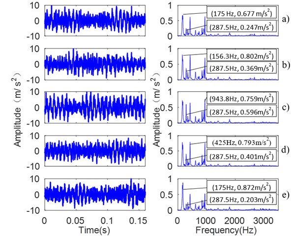
The vibration signals are collected in different pedestal looseness extents, such as T1 (all bolts tightened), T2 (1 bolt looseness), T3 (two bolts looseness), T4 (3 bolts looseness) and T5 (4 bolts looseness). When the number of loose bolts increases, the pedestal looseness extent strengthens. Fig. 1 shows the collected vibration signals and its spectrum of the five kinds of looseness extents.
Fig. 1 shows that there is difference among the vibration signal and its spectrum, for example the amount of spectrum energy, the position change of main frequency band and the decentralization or centralization degree of the spectrum. Fig.1 shows that the dominant frequency is 175 Hz, 156.3 Hz, 943.8 Hz, 425 Hz and 175 Hz respectively, and the dominant frequency amplitude is 0.677 m/s2, 0.802 m/s2, 0.759 m/s2, 0.793 m/s2 and 0.872 m/s2 respectively, the amplitude at 287.5 Hz is 0.247 m/s2, 0.369 m/s2, 0.596 m/s2, 0.401 m/s2 and 0.203 m/s2 respectively.
Fig. 2The probability density function in 5 kinds of looseness extent
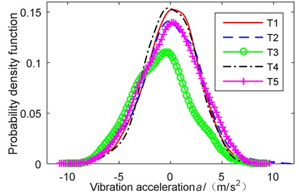
In order to further observe the characteristics of different looseness extents, the probability density function is calculated as shown in Fig. 2. The waveform of probability density function is different with different looseness ex-tents of pedestal, for example degree of asymmetry of probability density function, the peak value of density distribution curve at the average and so on.
Overall, the characteristics of vibration signal are changed with the change of the pedestal looseness extent, and the different pedestal looseness extents are characterized by different characteristics of vibration signal and its spectrum.
2.2. Looseness extent feature extraction and looseness extent feature set construction
The pedestal looseness extent of rotating machinery can be visibly characterized by time-frequency characteristics of vibration signal, but it difficult to automatic recognition by pattern recognition algorithm. In order to realize quantitative characterization of pedestal looseness extent and easily implement intelligent recognition, multiple features are extracted to construct origin looseness extent feature set. To reflect the change of the characteristic of the vibration signal as comprehensive as possible, integrated vibration signal time and frequency domain information, 29 time-frequency parameters are extracted. 15 time-domain parameters are extracted from vibration time-domain signal such as maximum amplitude, average amplitude, root mean square, shape factor, kurtosis index, crest factor, impulse factor, clearance factor, skewness index and so on. And, 14 frequency-domain parameters are extracted from frequency spectrum such as average frequency amplitude, centroid frequency, mean-square frequency, frequency variance, root mean square frequency and so on. Finally, we construct 15 feature parameters in time-domain and 14 feature parameters in frequency-domain as provided in Table 1, and further combine them into a 29-dimensional time-frequency feature parameter set in order to fully and reliably obtain the pedestal looseness extent features. Also, the origin looseness extent feature set is obtained.
In Table 1, represents the time series of a signal, 1, 2,…, , where is a sampling number. represents the frequency spectrum of , 1, 2,…, , where is spectrum line number. is the frequency of the -th spectrum line. represents the mean value of the . Time domain feature parameters - represent the amplitude and energy of the time domain signal; - denote the distribution situation of time series of the signal. Frequency domain feature parameters characterizes the spectrum energy; - characterize the position change of main frequency band; - characterize the decentralization or centralization degree of frequency spectrum.
Table 1The time-frequency feature parameters
No. | Feature parameter expression | No. | Feature parameter expression | No. | Feature parameter expression | No. | Feature parameter expression |
Compared with single domain signal feature extraction, the 29-dimensional time-frequency domain feature set has three advantages as explained below: 1) it is more benefit for pattern recognition than classic spectrum analysis method. 2) It is more comprehensive than single time-domain or single frequency-domain feature extraction method to reflect the characteristics of looseness extent. 3) It is more sensitive to the change of looseness extent characteristics than STFT, WVD, wavelet decomposition and EMD.
2.3. Looseness extent sensitive feature selection and the looseness extent sensitive feature set construction
The looseness extent sensitivity of each feature from origin looseness extent feature set is different, the non-sensitive feature and poor sensitivity feature are not only bound to affect the looseness characterization capabilities of the feature set but also interfere with the recognition results. Therefore, the sensitive feature for pedestal looseness extent must be selected to construct the looseness extent sensitive feature set, which characterization capabilities is stronger than origin looseness extent feature set, and the recognition accuracy will be improved.
The scatter matrix includes between-class scatter matrix and within-class scatter matrix [23, 24], the between-class scatter value and within-class scatter value could be calculated by the two scatter matrix. The identifiability of different feature classes is reflected by the between-class scatter value, the larger the between-class scatter value is, the better identifiability of the feature is. The clustering characteristic of the same feature classes is reflected by the within-class scatter matrix, the smaller the within-matrix scatter value is, the better clustering characteristic of the feature is. If the between-class scatter value is larger and the within-class scatter value is smaller for the feature, the identifiability of feature will be better for different looseness extent feature sets, and the clustering characteristic of the feature will be better too for the same looseness extent feature set, then, feature’s recognition capability will be stronger for different looseness extents of pedestal, and the looseness sensitivity of the feature will be better. Therefore, the looseness sensitivity index algorithm is designed based on between-class scatter matrix and within-class scatter matrix, according to the feature’s characteristics of reflecting the identification and the degree of clustering. At the same time the looseness extent sensitive features are able to select from origin looseness extent feature set to construct the looseness extent sensitive feature set.
There are class looseness samples of different looseness extents, including sample number each class. For origin high-dimensional feature set, , is number of dimension.
The within-scatter matrix as follows:
where is mean of the th class, is the mean of total samples.
The between-scatter matrix as follows:
where is the th eigenvalues of th class.
Then, the and are calculated, is the trace of the matrix. is average measurement of characteristic variance for all feature classes, is one of average measurement of average distance between global mean value and mean of each class.
Different looseness samples can be identified because they are located in different regions of the feature space. The larger the distance of these regions is, the better identifiability is. So, the algorithm of the looseness sensitivity index is designed as follows:
Obviously, the value of will be larger, if value of is larger or value of is smaller. The looseness sensitivity index reflect the feature’s recognition capability. The larger the value is, the stronger the recognition capability is. Also the smaller the value is, the weaker the recognition capability is.
The looseness extent sensitive feature is selected by the value of . The information is more overall if more features are selected, and it is useful to improve the recognition accuracy. But, the non-sensitive feature or poor sensitivity feature will be brought into feature set if the too many features are selected, the recognition accuracy will be affected. So, it is very important to decide how many features are selected. First of all, the looseness sensitivity index of each feature is calculated, (1, 2,…, ). Secondly, , the mean of all looseness sensitivity index is calculated. Finally, the looseness extent sensitive features are selected which sensitivity index , and the looseness extent sensitive feature set is constructed.
3. Dimensionality reduction of high-dimensional looseness sensitive feature set based on linear local tangent space alignment (LLTSA)
3.1. Problem description
Consider a looseness samples set ( is the number of all looseness samples) for training and test with noise from which exists an underlying nonlinear manifold () of dimension . Moreover, suppose isembedded in the ambient Euclidean space , where . The problem that dimension reduction with LLTSA solves is finding a transformation matrix which maps the looseness sample set in to the set in as follows:
where is the centering matrix which is used to improve the aggregation of nearest neighbors set of each sample , and is the identity matrix, is an -dimensional column vector of all ones, is the underlying -dimensional nonlinear manifold of .
3.2. The algorithm of LLTSA
Given the data set obtained by treating with Principal Component Analysis, for each point , its nearest neighbors by a matrix . In order to ensure the local structure of each , local linear approximation of the data points in is calculated with tangent space as follows:
where , is an orthonormal basis matrix of the tangent space and has eigenvalues of corresponding to its largest eigenvalues, and is defined as:
where is the local coordinate corresponding to the basis . Now, we can construct the global coordinates , 1, 2,…, , in based on the local coordinate , which represents the local geometry as follows:
where is the mean of the various , is a local affine transformation matrix that needs to be determined, and is the local reconstruction error. Letting and , we have:
To preserve as much of the local geometry as possible in the low dimensional feature space, we intend to find and to minimize the reconstruction errors as follows:
Therefore, the optimal affine transformation matrix has the form , and , where is the Moor-Penrose generalized inverse of .
Let and be the 0-1 selection matrix, such that , then the objective function is converted to this form:
where , and with According to the numerical analysis in [17], Wi can also be written as follows:
where is the matrix of eigenvectors of corresponding to its largest eigenvalues. To uniquely determine , we impose the constraint . Considering the map , the objective function has the ultimate form:
where . It is likely to be proved that the above minimization problem can be converted to solving a generalized eigenvalue problem as follows:
Let the column vectors , ,…, be the solutions of Eq. (13), ordered according to the eigenvalues, . Thus, the transformation matrix which minimizes the objective function is as follows:
In the practical problems, one often encounters the difficulty that is singular. This stems from the fact that the number of data points is much smaller than the dimension of the data. To attach the singularity problem of , we use the PCA to project the data set to the principal subspace. In addition, the preprocessing using PCA can reduce the noise. is applied to denote the transformation matrix of PCA.
Therefore, the ultimate transformation matrix is as follows: and .
Because of LLTSA’s good clustering performance, -dimensional looseness feature set outputted by LLTSA from high-dimensional looseness extent sensitive feature set . The low-dimensional looseness extent feature set has better identifiability than high-dimensional looseness extent sensitive set , and the features of are mutually independent, so the set is good for pattern recognition. The set is inputted into Weight nearest neighbor classifier for looseness extent recognition.
4. Pedestal looseness extent recognition by weigh nearest neighbor classifier (WKNNC) and the looseness extent recognition process
4.1. Looseness extent recognition by WKNNC
In order to finally realize pedestal looseness extent automatic recognition, the low-dimensional looseness extent sensitive feature set output by LLTSA serves should be recognized by classifier. The simplicity of nearest neighbor classifer (KNNC) algorithm makes it easy to implement. The KNNC has no complex training process, compared with other classification algorithms such as support vector machine, neural network and decision tree. It directly uses the local information of the classified data to form the final classification decision, which improves its efficiency of computation, makes it easy to realize and be widely used. But, it suffers from poor classification performance when samples of different classes overlap in some regions in the feature space, and its result is affected by the neighborhood size of , it has poor stability. Therefore, the Weight nearest neighbor classifier (WKNNC) [21] is useful for overcoming the shortcomings of KNNC. The WKNNC is an improvement of KNNC, it not only has the all advantages of KNNC, but also is insensitive the neighbor size of and better robustness. So, the WKNNC is used for pedestal looseness extent recognition.
Given a training set , consisting of samples, the class label of each sample is known, . The class label of testing sample need to be identified. The general idea of WKNNC is summarized as follows: for given testing sample , its nearest neighbors are selected from the training samples. The class label of testing sample is identified based on the class label of the nearest neighbors. The target of classification is to make the classification error minimum. And for each value , the classification error is as follows:
where is the probability of classified as , is error of class label classified as . The all misclassification errors set by WKNNC are same as follows:
Then, the calculation steps of the WKNNC are described as follows:
Step 1: The Euclidean distance between the testing sample and the training sample is defined as:
The nearest neighbor samples are selected from training samples based on the value of , denoted as , ,…, .
Step 2: The sample is selected from the nearest neighbor samples, which Euclidean distance with is maximum, the maximum Euclidean distance is denoted . Then, the is used to standardize the Euclidean distance between the other nearest neighbor samples and as follows:
where is the standard Euclidean distance.
Step 3: Using Gauss kernel function, the are transformed into similar probability between and as follows:
Step 4: The posterior probability that belongs to the class label ( 1, 2,…, ) is calculated based on the similar probability between and the nearest neighbor samples, the is as follows:
then, the most likely classification results are obtained as follows:
According to the similarity degree between the nearest neighbor samples and the testing sample , the WKNNC gives different weights to the nearest neighbor samples, which makes the classification results of the testing sample more close to the similar degree of training sample. Therefore, the WKNNC is insensitive the neighbor size of , and the robustness of the results for the looseness extent identification is better.
4.2. Looseness extent recognition process
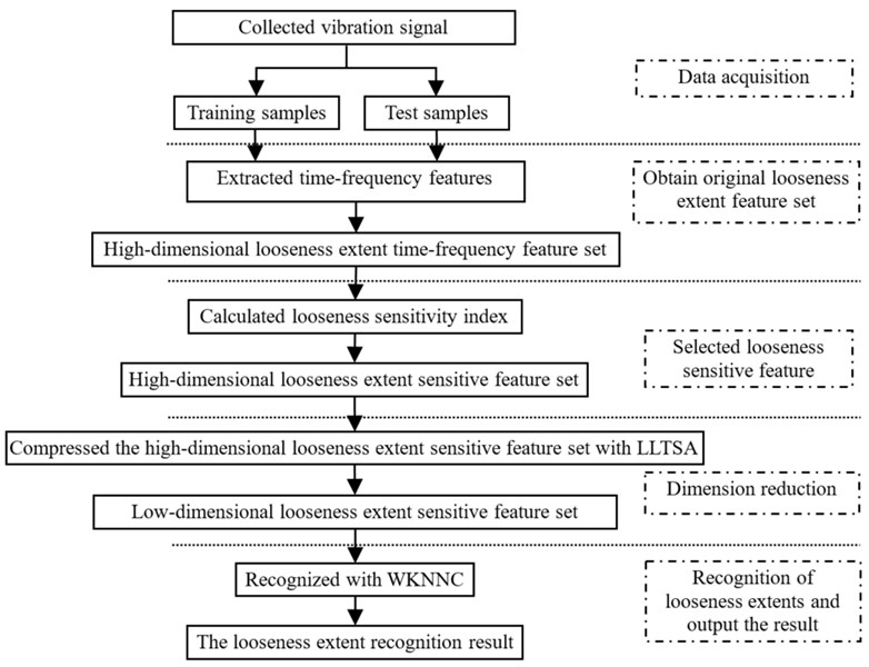
According to above preparation, the flowchart of the proposed method is shown in Fig. 3, the steps of the method are described as follows:
Step 1: data acquisition. The vibration signal is collected, and corresponding frequency spectrum is calculated, the training samples and test samples are obtained.
Step 2: extracted original features and constructed the original looseness extent feature set. 15 time-domain parameters are extracted from vibration signal, and 14 frequency-domain characteristic parameters are extracted from frequency spectrum, then 29-dimensional time-frequency looseness extent feature set is constructed by fusing the 14 time-domain parameters and 15 frequency-domain parameters.
Step 3: selected looseness sensitive feature and constructed looseness extent sensitive feature set. The looseness sensitivity index of each feature is calculated, ( 1, 2,…, ). Secondly, , the mean of all looseness sensitivity index is calculated. Then, the looseness features are selected which sensitivity index , and the looseness extent sensitive feature set is constructed.
Step 4: dimension reduction. The high-dimensional looseness extent sensitive feature set are compressed to low-dimensional looseness extent sensitive feature set with LLTSA. The low dimension and good classification performance feature set is obtained.
Step 5: recognition of looseness extents and output the recognition result. The low-dimensional feature set is inputted into WKKNC for looseness recognition, and the pedestal looseness extent recognition for rotating machinery is realized.
Fig. 3The flowchart of the proposed method
5. Application of the proposed method and discussion
5.1. Experiment set up and signal acquisition
In this study, a pedestal looseness experiment of rotating machinery is performed to verify the effectiveness of the proposed looseness extent recognition method. The test rig is constructed as shown in Fig. 4.
Fig. 4Field installation diagram and test diagram. (Notes:1, 2,…, 10 are the serial number of the connecting bolt for embedded steel plate)

The embedded steel plate is fixed on the top of the tunnel by 10 bolts, and the installing bracket of fan is installed in the embedded steel plate. Pedestal looseness extent is simulated by different number of loose bolts, when the number of loose bolts increases, the pedestal looseness extent strengthens. At the test point 1 and test point 2, the speed of fan is 1500 r/min, the vibration signals of 5 kinds of looseness extent are collected, such as T1 (all bolts tightened), T2 (1 bolt looseness), T3 (two bolts looseness), T4 (3 bolts looseness) and T5 (4 bolts looseness), are shown in Table 2. Fig. 1 shows the collected vibration signal and its spectrum of the five kinds of looseness extents, it only shows time domain waveform of first 4096 points and corresponding spectrum in the frequency range of 0-5000 Hz, collected at the test point 1. The complete sensor selection and distribution scheme are shown in Table 3.
Table 2The looseness extents of pedestal
Looseness extent | Description |
T1 | All bolts tightened |
T2 | 1 bolt looseness (bolt 8 looseness, others tightened) |
T3 | 2 bolts looseness (bolt 7 and 9 looseness, others tightened) |
T4 | 3 bolts looseness (bolt 6,8 and 10 looseness, others tightened) |
T5 | 4 bolts looseness (bolt 1,4,6 and 9 looseness, others tightened) |
Table 3The main parameters of the experiment
Serial number | Parameter/device | Value/ type |
1 | Accelerometer | PCB 352C03 |
2 | Sensitivity of the accelerometer | 1.031 mV/ m·s-2 |
3 | Frequency range of the accelerometer | 0.5 to 15000 Hz |
4 | Data acquisition card | NI 9234 |
5 | Data acquisition system | DAQ3.0 |
6 | Sampling frequency | 25.6 kHz |
7 | Sampling points | 100k |
5.2. Experimental results and analysis
2048 continuous data were intercepted from each sample as time series for looseness extent, then, we can obtain 100 samples in each of looseness extent. We randomly select just 20 samples out of the 100 acquired samples as the training samples, and randomly select 20 samples out of the remaining 80 samples as testing samples. Application of the proposed method to recognize the looseness extent of pedestal.
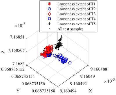
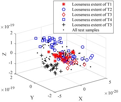
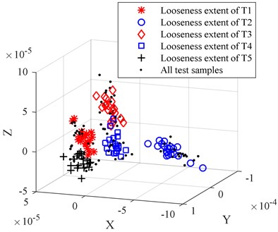
In order to compare the dimension reduction and redundant treatment effect of PCA, the LPP, the LDA, and the LLTSA method are used to reduce the dimension for origin looseness extent feature set. To be comparable, the dimensions of PCA, LPP, LDA and LLTSA are set to 3. The comparison of dimension reduction results is shown in Fig. 5(a)-(d).
By comparing Figs. 5(a)-(d) we can find that the PCA-based data dimension reduction method cannot effectively separate the high dimension looseness feature set, the looseness extent of T2 is separated, but there is still serious aliasing, which will affect the accuracy of the WKNNC looseness recognition effect. The LPP-based data dimension reduction method can partly separate the different looseness feature sets, there are still some data mixed together, the looseness extent of T1, looseness extent of T3 and looseness extent of T4 mixed together. The LDA-based data dimension reduction method can’t separate feature sets from the looseness extent of T1, the looseness extent of T2 and the looseness extent of T3. The LLTSA-based data dimension reduction method works better than the PCA, LPP and LDA methods, but the looseness extent of T3 and the looseness extent T4 don’t completely separated, and the clustering performance is not good enough.
The looseness sensitivity index of 20 features is calculated as shown in Table 4, and the mean of the sensitivity index 12.352. Then, 9 features (bolded part of the Table 4) that the sensitivity index are selected to construct the looseness sensitive feature set.
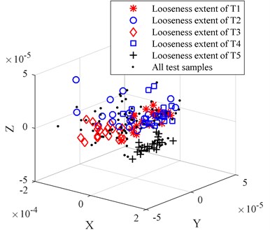
In order to compare the characterization capabilities between the origin looseness extent feature set and the looseness extent sensitive feature set, the looseness extent sensitive feature set is inputted into LLTSA to reduce the dimension, the dimensions of LLTSA is set to 3. The result is shown in Fig. 6.
By comparing Fig. 5(d) and Fig. 6 we can find that the result of Fig. 6 is better than result of Fig. 5(d). The 5 different looseness extents are completely separated in Fig. 6, and the better clustering performance is obtained.
In order to compare the recognition accuracy of origin looseness extent feature set and looseness extent sensitive feature set, and the recognition accuracy of dimension reduction methods such as PCA, LPP, LDA and LLTSA, the origin looseness extent feature set and looseness extent sensitive feature set are respectively inputted PCA, LPP, LDA and LLTSA to reduce dimension. The results of dimension reduction are respectively inputted WKNNC to recognize the looseness extent. The dimensions are set to 3, and the nearest neighbor is set to 9. The measurement of computation time was made in the follows computer configuration environment: 10G RAM, 3.4 GHz Inter Core i7-3770 CPU, 64-bit Operating System and MATLAB R2015b.
Fig. 5The comparison of dimension reduction results for origin looseness extent feature set
a) The dimension reduction results of PCA
b) The dimension reduction results of LPP
c) The dimension reduction results of LDA
d) The dimension reduction results of LLTSA
The comparison results are shown in Table 5. In Table 5, the recognition accuracy rate is defined as:
where represents the total number of testing samples, represents the number of testing samples correctly recognized, represents the pedestal looseness extent of the testing samples, 1, 2,…, 5.
The average recognition accuracy rate can be expressed as:
Table 4The sensitivity index
Number No. | Sensitivity index | Number No. | Sensitivity index | Number No. | Sensitivity index | Number No. | Sensitivity index | Number No. | Sensitivity index |
10.353 | 5.857 | 3.257 | 9.566 | 32.803 | |||||
9.481 | 0.072 | 3.562 | 43.857 | 18.232 | |||||
8.782 | 2.585 | 3.052 | 9.574 | 4.0230 | |||||
10.489 | 0.079 | 28.247 | 2.289 | 11.627 | |||||
5.857 | 3.996 | 24.299 | 1.820 | 13.847 | |||||
10.489 | 13.786 | 34.497 | 31.834 |
Fig. 6The dimension reduction results of LLTSA for looseness extent sensitive feature set
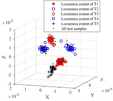
Table 5The comparison of recognition accuracy
The kinds of feature set | Reduction dimension methods | (%) | (%) | (%) | (%) | (%) | (%) | Computation time (s) |
Origin looseness extent feature set | PCA | 45 | 50 | 80 | 75 | 95 | 69 | 0.29 |
LPP | 50 | 45 | 95 | 85 | 100 | 75 | 0.21 | |
LDA | 60 | 75 | 70 | 60 | 90 | 71 | 0.19 | |
LLTSA | 80 | 95 | 80 | 90 | 85 | 86 | 0.46 | |
Looseness extent sensitive feature set | PCA | 75 | 90 | 75 | 55 | 85 | 76 | 0.20 |
LPP | 70 | 85 | 80 | 95 | 100 | 86 | 0.18 | |
LDA | 75 | 95 | 80 | 85 | 90 | 85 | 0.16 | |
LLTSA | 95 | 100 | 95 | 100 | 95 | 97 | 0.37 |
Table 5 indicates that the average recognition accuracy rate of test samples achieved by looseness extent sensitive feature set is 97 %, which is higher than that of the origin looseness extent feature set, when the dimension reduction method remains unchanged. The reason for the looseness extent sensitive feature set don’t include the non-sensitive feature and poor sensitivity feature, which enhanced the ability to characterize the pedestal looseness, and improved the recognition accuracy rate. Also, we can see that after the LLTSA-based dimension reduction method, the accuracy of looseness extent recognition improved significantly, much higher than the other dimension reduction methods, because LLTSA has advantage of suitable nonlinear reduction and more superior clustering performance, it is conducive to the recognition. The computation time of LLTSA is 0.46 s, which is more other dimension reduction methods, but it also very fast, doesn’t affect the engineering applications. Also, we can find that the computation time is reduced, when using looseness extent sensitive feature set to recognize and the dimension reduction method remain unchanged.
Next, recognition accuracy of WKNNC is compared with KNNC, where the nearest neighbor size of WKNNC and KNNC is also set as 3-20, the dimension reduction method is LLTSA. Also, the origin looseness extent feature set and the looseness extent sensitive feature set are used to compare. The recognition accuracy rate curve with the nearest neighbor size are as shown in Fig. 7, then, for each curve, the average recognition accuracy rate, standard deviation and peak-peak value are calculated as shown in Table 6.
Fig. 7The comparison of recognition results
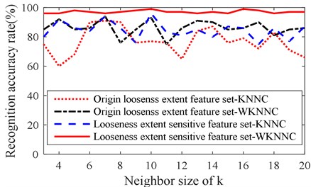
Table 6Recognition result analysis
Origin looseness extent feature set-KNNC | Origin looseness extent feature set-WKNNC | Looseness extent sensitive feature set-KNNC | Looseness extent sensitive feature set-WKNNC | |
Average recognition accuracy rate (%) | 77 | 86.17 | 84.5 | 97.06 |
Standard deviation (%) | 9.16 | 5.18 | 5.81 | 0.99 |
Peak-peak value (%) | 31 | 19 | 21 | 3 |
Fig. 7 and Table 6 show that the recognition accuracy rate of WKNNC is higher than KNNC, the standard deviation and peak-peak value of WKNNC are less than KNNC, because the nearest neighbor samples are given different weights, which makes the classification results of the testing sample more close to the similar degree of training sample, which also prove that the WKNNC is insensitive the neighbor size of , having better stability and robustness than KNNC. The recognition accuracy rate based-looseness extent sensitive feature set is higher than the based-origin looseness extent feature set when the pattern recognition algorithm is same, which confirm again that the characterization capabilities of looseness extent sensitive feature set is stronger than origin looseness extent feature set. The standard deviation and peak-peak value based-looseness extent sensitive feature set is smaller than the based-origin looseness extent feature set when the pattern recognition algorithm is same, which confirm that the stability of characterization method based-looseness extent sensitive feature set is better than based- origin looseness extent feature set, and the clustering performance of looseness extent sensitive feature set is better too. Table 5, Fig. 7 and Table 6 show that the recognition accuracy rate of the proposed method is higher than other method, and it insensitive the neighbor size of , having better stability and robustness.
This application example demonstrates well the performance of the proposed method which comprehensively uses characteristics of vibration signal to characterize the pedestal looseness extent, extracts time-frequency feature to construct origin looseness extent feature set, obtains looseness extent sensitive feature set to enhance the characterization capabilities, reduce dimension with LLTSA, and recognize looseness extent with WKNNC. The results conform the proposed method can recognize the pedestal looseness extent. Also, the feasibility and validity of the proposed method are verified by experimental results.
6. Conclusions
A pedestal looseness extent recognition method for rotating machinery based on vibration sensitive time-frequency feature and manifold learning has been proposed in this paper.
1) When the rotating machinery pedestal is loose, the structure dynamic characteristics of the rotating machinery will be change, the vibration signal and its spectrum will be change too. Then, pedestal looseness extent of rotating machinery is exactly characterized by the characteristics of vibration signal and its spectrum.
2) The time-frequency features are extracted to construct the origin looseness extent feature set, which includes 15 time-domain parameters and 14 frequency-domain parameters. Then, the origin looseness extent feature set has realized quantitative characterization of pedestal looseness extent, which easily implement intelligent diagnosis.
3) The algorithm of looseness sensitivity index is designed, the non-sensitive feature and poor sensitivity feature are removed from origin looseness feature set. Then, the looseness extent sensitive feature set is obtained, which characterization capabilities and clustering performance are better than origin feature set. A manifold learning algorithm LLTSA has excellent clustering and dimension reduction characteristics, and is perfectly suitable to reduce non-linear feature set. It is used to reduce the high-dimensional and non-linear looseness extent sensitive feature set.
4) The WKNNC gives different weights to the nearest neighbor samples based on the similarity degree between the nearest neighbor samples and the test samples. So the WKNNC is insensitive the neighbor size of , and the robustness of the results for pedestal looseness extent recognition is better.
5) The proposed method makes use of the advantage of all parts and together to realize pedestal looseness extent recognition of rotating machinery and obtain better recognition accuracy and efficiency. The feasibility and performance of the proposed method was proved by successful pedestal looseness extent recognition application in a fan pedestal.
6) The proposed method could be used for identification and classification of other rotating machinery faults. For example, rotating bearing faults like inner race crack, outer race crack and ball crack, etc. It must be noted that the training samples and testing samples should be from the same operating conditions, because the time-frequency features are difficult to effectively characterize the faults of rotating machinery when the operating conditions are different, such as rotor speed and load.
It should be pointed out that the pedestal looseness extent could be effectively recognized, but there is a problem to solve. For example, we can be sure that there are two bolt loose, but it is difficult to determine which of the two bolts, so we need to manually check each bolt when maintain the equipment. So, it is interesting to study the problem in the future.
References
-
Se Camby M. K., Lee Eric W. M., Lai Alvin C. K. Impact of location of jet fan on airflow structure in tunnel fire. Tunnelling and Underground Space Technology, Vol. 27, Issue 1, 2012, p. 30-40.
-
Costantino Antonio, Musto Marilena, Rotondo Giuseppe, et al. Numerical analysis for reduced-scale road tunnel model equipped with axial jet fan ventilation system. Energy Procedia, Vol. 45, 2014, p. 1146-1154.
-
Qin Zhaoye, Han Qinkai, Chu Fulei Bolt loosening at rotating joint interface and its influence on rotor dynamics. Engineering Failure Analysis, Vol. 59, 2016, p. 456-466.
-
Zhang Yanping, Huang Shuhong, Hou Jinghong, et al. Continuous wavelet grey moment approach for vibration analysis of rotating machinery. Mechanical Systems and Signal Processing, Vol. 20, Issue 5, 2006, p. 1202-1220.
-
Lee Seung-Mock, Choi Yeon-Sun Fault diagnosis of partial rub and looseness in rotating machinery using Hilbert-Huang transform. Journal of Mechanical Science and Technology, Vol. 22, Issue 11, 2008, p. 2151-2162.
-
Wu T. Y., Chung Y. L., Liu C. H. Looseness Diagnosis of rotating machinery via vibration analysis through Hilbert-Huang transform approach. Journal of Vibration and Acoustics, Vol. 132, Issue 3, 2010, p. 031005.
-
Wu Tian-Yau, Hong Huei-Cheng, Chung Yu-Liang A looseness identification approach for rotating machinery based on post-processing of ensemble empirical mode decomposition and autoregressive modeling. Journal of Vibration and Control, Vol. 18, Issue 6, 2011, p. 796-807.
-
Nembhard Adrian D., Sinha Jyoti K., Yunusa-Kaltungo A. Development of a generic rotating machinery fault diagnosis approach insensitive to machine speed and support type. Journal of Sound and Vibration, Vol. 337, Issue 17, 2015, p. 321-341.
-
Muralidharan V., Sugumaran V. Roughset based rule learning and fuzzy classification of wavelet features for fault diagnosis of monoblock centrifugal pump. Measurement, Vol. 46, Issue 9, 2013, p. 3057-3063.
-
Su Zuqiang, Tang Baoping, Deng Lei, et al. Fault diagnosis method using supervised extended local tangent space alignment for dimension reduction. Measurement, Vol. 62, 2015, p. 1-14.
-
Yang C. Y., Wu T. Y. Diagnostics of gear deterioration using EEMD approach and PCA process. Measurement, Vol. 61, 2015, p. 75-87.
-
He Fei, Xu Jinwu A novel process monitoring and fault detection approach based on statistics locality preserving projections. Journal of Process Control, Vol. 37, 2016, p. 46-57.
-
Akbari Ali, Khalil Arjmandib Meisam An efficient voice pathology classification scheme based on applying multi-layer linear discriminant analysis to wavelet packet-based features. Biomedical Signal Processing and Control, Vol. 10, 2014, p. 209-223.
-
Li Feng, Wang Jiaxu, Tang Baoping, et al. Life grade recognition method based on supervised uncorrelated orthogonal locality preserving projection and k-nearest neighbor classifier. Neurocomputing, Vol. 138, Issue 22, 2014, p. 271-282.
-
Souza Roberto, Rittner Letícia, Lotufo Roberto A comparison between k-Optimum Path Forest and k-Nearest Neighbors supervised classifiers. Pattern Recognition Letters, Vol. 39, Issue 1, 2014, p. 2-10.
-
Saravanan N., Kumar Siddabattuni V. N. S., Ramachandran K. I. Fault diagnosis of spur bevel gear box using artificial neural network (ANN), and proximal support vector machine (PSVM). Applied Soft Computing, Vol. 10, Issue 1, 2010, p. 344-360.
-
Moosavia S. S., Djerdira A., Ait-Amiratb Y., et al. ANN based fault diagnosis of permanent magnet synchronous motor under stator winding shorted turn. Electric Power Systems Research, Vol. 125, 2015, p. 67-82.
-
Salahshoor Karim, Kordestani Mojtaba, Khoshrob Majid S. Fault detection and diagnosis of an industrial steam turbine using fusion of SVM (support vector machine) and ANFIS (adaptive neuro-fuzzy inference system) classifiers. Energy, Vol. 35, Issue 12, 2010, p. 5472-5482.
-
Muralidharan a V., Sugumaran V., Indira V. Fault diagnosis of monoblock centrifugal pump using SVM. Engineering Science and Technology, Vol. 17, Issue 3, 2014, p. 152-157.
-
Zhang Tianhao, Yang Jie, Zhao Deli, et al. Linear local tangent space alignment and application to face recognition. Neurocomputing, Vol. 70, Issues 7-9, 2007, p. 1547-1553.
-
Lei Yaguo, Zuo Ming J. Gear crack level identification based on weighted K nearest neighbor classification algorithm. Mechanical Systems and Signal Processing, Vol. 23, Issue 5, 2009, p. 1535-1547.
-
Chen Lifei, Guo Gongde Nearest neighbor classification of categorical data by attributes weighting. Expert Systems with Applications, Vol. 42, Issue 6, 2015, p. 3142-3149.
-
Wang Yuli, Chakrabarti Amitabha, Sorensen Christopher M. A light-scattering study of the scattering matrix elements of Arizona road dust. Journal of Quantitative Spectroscopy and Radiative Transfer, Vol. 163, 2015, p. 72-79.
-
Yao Chao, Lu Zhaoyang, Li Jing, et al. An improved Fisher discriminant vector employing updated between-scatter matrix. Neurocomputing, Vol. 173, 2016, p. 154-162.
Cited by
About this article
This research was supported by the National Natural Science Foundation of China (Project No. 51305471, No. 51405048, No. 51505048), China Postdoctoral Science Foundation (Project No. 2014M560719), Chongqing Research Program of Basic Research and Frontier Technology (Project No. cstc2014jcyjA70009), Science and Technology Research Project of Chongqing Education Commission (Project No. KJ1400308, No. KJ1500516), National Scholarship Project (No. 201408505081). Finally, the authors are very grateful to the anonymous reviewers for their helpful comments and constructive suggestions.
Renxiang Chen contributed to the conception of the study and proposed the method. Zhiyan Mu designed and performed the experiments. Lixia Yang performed the data analyses and wrote the manuscript. Xiangyang Xu helped perform the analysis with constructive discussions. Xia Zhang played an important role in interpreting the results.
