Fault diagnosis of rotating machinery based on time-frequency decomposition and envelope spectrum analysis

2.1. Improved EEMD

EMD was first designed by Huang et al. to decompose a complex signal into a series of IMF decompositions [19]. Before using EMD to process signals, three assumptions are considered: (1) the signal must have at least two extreme points, i.e., one maximum and one minimum; (2) the characteristic time scale is defined by the time lapse between extreme points and (3) if the data are totally devoid of extrema but contain only inflection points, then they can be differentiated one or more times to reveal the extrema.

From the EMD method, a complex signal $x\left(t\right)$ can be composed into the following form:

where $c_i\left(t\right)$ is the $i$th IMF composition and $r_n\left(t\right)$ is the residue.

For these IMF compositions of the EMD, they are all nearly orthogonal functions and each one represents a simple oscillation mode with physical meaning. Concurrently, the IMF also satisfies two conditions:

(1) For the whole data series, the number of extrema and zero crossings should be equal or differ at most by one.

(2) At any data point, the mean value of envelopes defined by local maxima and minima of original signal should be zero.

However, EMD has a major drawback of mode mixing, which means that a single IMF composition contains oscillations with observably disparate scales or the oscillations in a similar scale appearing in several IMFs at the same time [3]. To solve this problem, a new signal processing method named EEMD was proposed by Wu and Huang [20]. In this new signal processing method, white noise-added technology is employed and the mean values of these decomposition results of traditional EMD trials are treated as the final IMF compositions. Therefore, the complex signal $x\left(t\right)$ can be decomposed into the following form:

where ${\stackrel{-}{c}}_i\left(t\right)$ and ${\stackrel{-}{r}}_m\left(t\right)$ is the ensemble means of the corresponding IMF decompositions and residues in a series decomposition EMD trials.

Although EEMD can assist in resolving the mode mixing problem of EMD and obtain more meaningful components, the non-IMF problem is still a major drawback when attempting to develop accurate decomposition effects. Based on this issue, Huang and Wu [20] provide guidance towards eliminating these imperfections involving another round of sifting on the IMFs produced by EEMD. All decomposition that results from traditional EMD can be regarded as well-IMFs. Therefore, EEMD and EMD can be combined to resolve the non-IMF problem to develop meaningful components for effective feature extraction based on the methods introduced in the literature [17, 18]. According to the decomposition theory of EEMD, the main frequency components in IMFs are lined from high to low, that is to say, the frequency of front IMF is higher than that of latter one. Different IMFs include various degree information indicating mechanical faults. At the same time, several new IMFs will also be obtained when using EMD to process the selected decomposition results of EEMD. Therefore, it is necessary to select an appropriate IMF to extract effective features.

According to above analysis, a new IEEMD, consuming less time than these methods in [17] and [18], is proposed for fault diagnosis of the bearings discussed in this paper. This method mainly includes two steps: processing the original vibration signals with traditional EEMD, and using EMD to resolve the decomposition results of EEMD where each step has an IMF selection task. In the first step, the appropriate IMF is selected processing by an EMD. For the second step, the IMF is selected for features. Except when the selected IMF is implemented, the remaining decomposition components are summed as the equivalent residue, which is then removed as noise. By utilizing the improved EEMD, we can cancel noise components from the original vibration signals. The procedure is shown as follows.

(1) Process the original vibration signal $x\left(t\right)$ with standard EEMD and develop a series of IMF components. In this step, the two parameters of EEMD are set as follows: the ensemble number is 100 and the appropriate amplitude of added white noise is 0.2 times the standard deviation of the signal.

(2) Calculate the energy values of these IMFs whose main frequency information is not less than rotating frequency. The IMF with the largest energy value is selected as useful information for further processing. At the same time, the other components are regarded as noise and cancel directly.

(3) Then the selected IMF is processed by traditional EMD, and a serious of new IMFs also can be obtained.

(4) The IMF calculated in step (3), having the largest energy values, is selected as the final IMF to calculate features by envelope spectrum analysis using a Hilbert transform.

2.2. Simulation analysis

To test the effectiveness of the proposed method for processing of complex signals, a number simulation experiment is carried out. In this simulation, each IMF of the EEMD is processed with the traditional EMD to show the improvement. The simulated digital signals are as follows:

where $T_1=$ 1000, $T_2=$ 0.25$i$ and $i=$ 1, 2, 3; $e\left(t\right)$ is noise.

Fig. 1The time domain waves of simulation signals

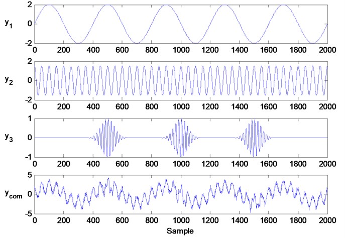
The time domain waves of simulation signals, as determined by Eq. (3), are plotted in Fig. 1. There are four types of compositions in the final simulation signal: (1) one sinusoidal signal, (2) one cosine signal, (3) one impulse signal and (4) noise. The primary frequencies are 5 Hz, 40 Hz and 100 Hz, which can be observed in Fig. 2. From this figure, we can see that the impulse signal is relative weaker than the sinusoidal and cosine signals. Concurrently, there are many other compositions with small amplitude distributed frequencies that are produced by noise.

Fig. 2The frequency domain waves of simulation signals

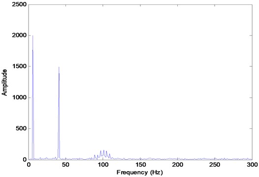
Fig. 3 shows the decomposition information of the traditional EMD. Directly observing the plots in Fig. 3, it can be concluded that the signal $y_1$ is able to decompose into $c_5$. Most of the components in $y_2$ are decomposed into $c_4$; however,$c_3$ not only includes much of the information contained in $y_3$, but also has significant noise interference and part of the information contained in $y_2$. For this type of phenomenon, a signal appears in two or more IMF components, and is the so-called mode mixing of EMD. Therefore, the traditional EMD cannot effectively resolve a complex signal.

Fig. 3The decomposition information of traditional EMD, in which the components c1 to c6 are IMFs and r is residual signal

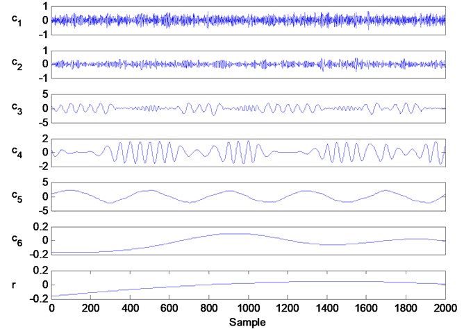
Fig. 4The decomposition information of traditional EEMD, in which the components c1 to c6 are the first six IMFs and the other decomposition information is not showed

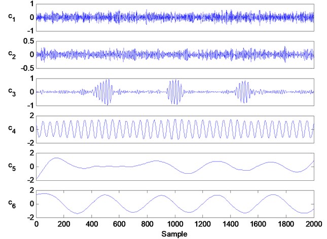
Fig. 4 shows the decomposition results of the EEMD process. According to this figure, we can see the main components of $y_3$, $y_2$ and $y_1$ are decomposed into $c_3$, $c_4$and $c_5$, respectively. Although $c_3$ includes some information regarding $y_3$ and $c_5$ also has some information regarding $y_1$, the decomposition results of EEMD are better than that of traditional EMD.

Fig. 5 shows the decomposed results of IEEMD. Per the operating procedure of IEEMD, the well-IMFs are handled from these decomposition components of traditional EEMD. In fact, it can be regarded as a denoising process. From these plots in Fig. 5, we can see that these singles are clearer than those in Fig. 4. At the same time, the signal components belonging to simulation signals contain more energy values than those of other IMFs. Then we can select this IMF with the largest energy value to extract features for fault diagnosis.

Fig. 5The decomposition information of IEEMD, in which the components c1 to c6 are the first six IMFs and the other decomposition information is not showed

3.1. Feature extraction

A bearing cannot smoothly work after a defect appears. Additionally, the impact to other components will also be collected by sensors. For different bearing faults, the main frequencies will vary and are defined as characteristic damage frequencies (CDFs). Generally, these CDFs are determined by shaft rotational speed and the structural parameters of a bearing, which can be calculated by [9]:

where $n$ is the speed of shaft; $f_{speed}$ is shaft rotational frequency; $f_{in}$, $f_{ball}$ and $f_{out}$ are CDFs of inner race fault, ball fault and outer race fault, respectively; $B$ and $P$ are ball and pitch diameter, respectively; $N$ is the number of balls; and $\theta$ is the angle of the load from the radial plane.

According to Eq. (4), if a bearing is under normal stress then the shaft rotational frequency component will be large. If one fault appears, the information of CDFs will increase. Therefore, the energies of a band frequency nearby, i.e., 1× ($f_{speed}$, $f_{in}$, $f_{ball}$ and $f_{out}$), 2× ($f_{speed}$, $f_{in}$, $f_{ball}$ and $f_{out}$) are computed as features.

When extracting features as above description, how to accurately find these frequency components of CDFs and shaft rotational frequency is also a thorny problem need to be solved. The theoretical values of CDFs will be different from their actual values because of following reasons: when rotating machinery working, its shaft rotational frequency will be fluctuations; at the same time, the used frequency resolution may also impact on the finding effect of CDFs and shaft rotational frequency. In order to extract sufficient fault impact information, a CDF finding algorithm is presented in this paper, and which mainly includes following steps:

First, calculate theoretical values of CDFs with Eq. (4), and which are marked as $f_{in}^{*}$, $f_{ball}^{*}$ and $f_{out}^{*}$. In this paper, the shaft rotational frequency for calculating CDFs is regarded as the set value when rotating machinery working. In actual production, a rotary machine usually has a preset rotating speed $f_{speed}^{*}$, although it may run with a speed which fluctuates within a certain range nearby $f_{speed}^{*}$.

Second, determine the searching radius of impact frequency and denote it as $f_{range}^{*}$. Further analysis of Eq. (4), we can find that CDF can be regarded as a factor times shaft rotational frequency. Therefore, we set $f_{range}^{*}=0.5\times f_{speed}^{*}$.

Third, find this frequency with maximal amplitude among the searching frequency interval which is defined as $\left[\begin{array}{cc}F-f_{range}^{*}& F+f_{range}^{*}\end{array}\right]$, and which is denoted as $F_{\mathrm{m}\mathrm{a}\mathrm{x}}$. In this step, F can be replaced by $f_{speed}$, $f_{in}$, $f_{ball}$ and $f_{out}$.

Final, calculate the energy of these frequency among ${[i\times F}_{max}-d,{i\times F}_{max}+d]$ as feature. In fact, $F_{max}$ can be treated as the most likely CDF or shaft rotational frequency information.

3.2. SVM based fault diagnosis

Typically, a complete fault diagnosis method includes three steps: signal collection, feature extraction by signal processing and fault decision. After extracting features from original vibration signals, the method for using these features for fault diagnosis is also an important step. SVM is presented from the statistical learning theory to solve binary classification issues based on the structural risk minimization principle [21-23]. Using a few feature samples, SVM can be trained. Therefore, SVM is employed to perform fault diagnosis based on the extracted features. In this study, the used SVM code was acquired from the LIBSVM open source code library maintained by the National Taiwan University [23] and the procedure for the proposed method is shown in Fig. 6.

Fig. 6Procedure of the proposed method

4.1. Experimental setup

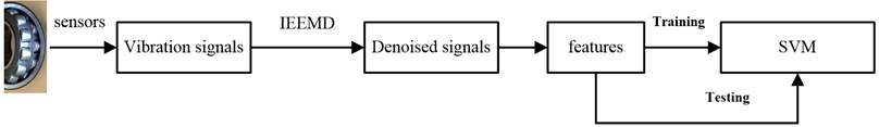
To test the effectiveness of the proposed method based on the EEMD, correlation analysis and SVM, an experimental study was implemented using vibration data sets from the bearing data center of Case Western Reserve University [24]. This simulator includes a 3-phase, 2 hp induction motor, a torque, rolling element bearings (6205-2RS JEM SKF) and a dynamometer. The test bearings were installed at the drive end to support the motor shaft. The bearing faults were all single point damages with fault diameters of 0.007 inches that were formed using electro-discharge machining methods. The sample frequency used was 12000 Hz and the corresponding vibration signals were collected by accelerometers using a 16 channel data recorder when bearings were rotating at a speed of 1797 rpm or 29.95 Hz. According to Eq. (4), we can get the theoretical values of $f_{in}$, $f_{ball}$ and $f_{out}$ are 162.2 Hz, 142.2 Hz and 107.3 Hz, respectively. In this study, the test conditions included normal operations and three types of faults including an inner race fault, a ball fault and an outer race fault. Fig. 7 shows the segmental vibration signals. According to the plots in Fig. 8, the difficulty of performing fault diagnosis solely based on the time domain information from the collected vibration signals can be observed.

Fig. 7The waves of vibration signals and their frequencies

4.2. Experimental results and discussion

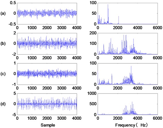
For a bearing, the vibration signal of inner race fault has the least useful information than for the other types of bearing faults. This is due to the fact that most of the energy from the useful information is lost after transferring from the inner race through ball bearings to the outer race and finally to the sensors. Therefore, the decomposition results of the vibration signals due to an inner race fault are shown in this study with a portion of the decomposition results shown in Fig. 8. In this figure, $c_1$ to $c_6$ are the first six IMFs of the EEMD, $C_{IMF}$ is the final IMF of the IEEMD and $E_1$ is the energy of $c_1$. Concurrently, the energy values of other IMFs are also described based on the form of ${k\times E}_1$.

From Fig. 8, we can see that $c_1$ has the largest energy value compared to the other decompositions of the EEMD. Therefore, $c_1$ is selected and processed with EMD. After processing by EMD, $c_1$ is decomposed into a new series of IMFs where the new IMFs may include various useful information. Therefore, the IMF with the largest energy value is selected for purpose of this study. The final IMF obtained by the IEEMD includes most of the energy belonging to $c_1$, that is to say, the proposed method can improve the decomposition results of the EEMD while resolving some noise. According to the principles of traditional EMD, the decomposition results are suitable IMFs. Therefore, the proposed IEEMD can solve the non-IMF problem of EEMD. Additionally, experimental verification can be found in Refs. [16, 17]. In this study, each feature is extracted from 4000 points from the vibration signal; hence, the length of the data segment processed by IEEMD is 4000 sampling values.

Fig. 8The decomposition results of inner race fault with IEEMD, in which c1 to c6 are the first six IMFs of EEMD, CIMF is the final IMF of IEEMD and E1 is the energy of c1

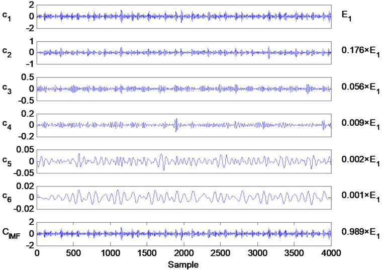
Fig. 9 shows the envelope spectrums of the selected IMF under consideration, where (a), (b), (c) and (d) show the data for bearings under normal conditions, an inner race fault, a ball fault and an outer race fault, respectively. From these plots, it can be concluded that different bearing conditions have various main frequencies components. For bearings working under normal conditions, the main frequency information is 33 Hz, which can be regarded as the shaft rotational frequency component, and the second peak frequency is 63 Hz. In Fig. 10(b), two peaks appear at frequencies 165 Hz and 327 Hz, which are close to $f_{in}$ and $2{\times f}_{in}$. Hence, the CDFs of an inner race fault can be easily observed from Fig. 9(b). In the same manner, the CDFs of the ball fault and the outer race fault can also be observed in Figs. 9(c) and 9(d), respectively. However, the frequency values of the peaks are not equivalent to theoretical values of the CDFs. Therefore, it is hard to extract effective features directly using these theoretical values of the CDFs. In order to extract as much information as possible from the CDFs, the energies of a frequency band around the CDFs are computed. In this study, the shaft rotational frequency is defined as the “CDF” normal and the bandwidth is set at 9 Hz, i.e., $d=$ 9. For each bearing condition, the energies of ${[f}_{cdf}-d,\mathrm{}{\mathrm{}f}_{cdf}+d]$ and ${[2f}_{cdf}-d,\mathrm{}{\mathrm{}2f}_{cdf}+d]$ are obtained. Therefore, two feature parameters will be calculated for each considered condition, i.e., the extracted feature is a vector with eight elements.

For this study, 100 samples are extracted from the decomposition results of the IEEMD using the Hilbert transform and envelope spectrum analysis. It is difficult to collect a very large data set for each individual condition of the rotating machinery. Therefore, 20 samples are randomly selected to construct the training set to design the SVM mode. The remaining 80 samples then are categorized as a test set for future testing. In the training step, the outputs of the SVM model for these samples under the conditions shown in Fig. 9(a), 9(b), 9(c) and 9(d) are identified as “1”, “2”, “3” and “4”, respectively. The other parameters of the SVM model are set as the default values. The default values themselves were obtained from Ref. [21].

Fig. 9The envelope spectrums of consideration conditions

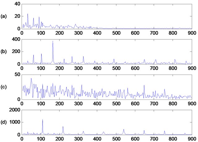
Fig. 10The test results of the proposed method

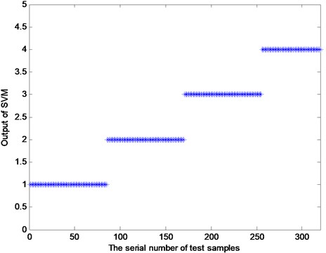
The test results are shown in Fig. 10. As shown in this figure, the outputs of the samples with Nos. 1-80 are “1”. The value of 1 indicates the test samples are all successfully diagnosed as normal and the test results precisely correspond to the real health conditions of the test samples. In the same fashion, the other test samples are all diagnosed accurately. Therefore, Fig. 10 shows that the propose method is effective for fault diagnosis of rotating machinery. Additionally, the IEEMD algorithm can be considered a satisfactory process.