Abstract
It is crucial to effectively and accurately diagnose the faults of rotating machinery. However, the high-dimensional characteristic of the features, which are extracted from the vibration signals of rotating machinery, makes it difficult to accurately recognize the fault mode. To resolve this problem, t-distributed stochastic neighbor embedding (t-SNE) is introduced to reduce the dimensionality of the feature vector in this paper. Therefore, the article describes a proposed method for fault diagnosis of rotating machinery based on local characteristic decomposition-sample entropy (LCD-SampEn), t-SNE and random forest (RF). First, the original vibration signals of rotating machinery are decomposed to a number of intrinsic scale components (ISCs) by the LCD. Next, the feature vector is obtained through calculating SampEn of each ISC. Subsequently, t-SNE is used to reduce the dimension of the feature vectors. Finally, the reconstructed feature vectors are applied to the RF for implementing the classification of the fault patterns. Two cases are studied based on the experimental data of the fault diagnoses of a bearing and a hydraulic pump. The proposed method can achieve a diagnosis rate of 98.22 % and 98.75 % for the bearing and the hydraulic pump, respectively. Compared with the other methods, the proposed approach exhibits the best performance. The results validate the effectiveness and superiority of the proposed method.
1. Introduction
Rotating machinery is widely used in many types of machine systems [1, 2]. If a failure occurs in rotating machinery, it may result in the breakdown of the machine system and major loss [3]. Therefore, fault diagnosis of rotating machinery has attracted increasing interest in recent years [4].
Rotating machinery under an abnormal state is usually accompanied by changes in vibration [5]. Therefore, fault detection via vibration monitoring has been proven to be an effective method of enhancing the reliability and safety of machinery.
Local characteristic-scale decomposition (LCD) is a type of data-driven and adaptive non-stationary signal decomposition method and hence is suitable for processing non-stationary signals, such as the vibration signals of rotating machinery [6, 7]. The LCD method can self-adaptively decompose vibration signals into a series intrinsic scale components (ISCs) and a residue with a shorter running time and a smaller fitting error.
To compress the scale of the fault feature vectors, appropriate entropy is usually employed. The appropriate entropy is an effective tool developed by Pincus [8] to determine the complexity of a time series. However, the appropriate entropy is based on the calculation model using a logarithm, which leads to it not being sensitive to small fluctuations of the complexity. To resolve this problem, Richman and Moorman [9] proposed the sample entropy (SampEn), which is a modified version of the appropriate entropy and is not dependent on a logarithm. SampEn can quantify the degree of the complexity in a time series and is insensitive to the data length and immunity to the noise in the data [10]. Therefore, the SampEn of different ISCs can be used to estimate the complexity at multiple time scales.
The LCD-SampEn generates a feature vector with a high dimension. Considering that the high dimensionality may result in feature redundancy and a waste of resources for subsequent calculation, it is necessary to reduce the dimensionality of the feature vector. Manifold learning methods are widely used as dimension reduction methods and can be divided into two types: linear methods and nonlinear methods. Linear manifold learning methods include principal component analysis (PCA) and multidimensional scaling; nonlinear manifold learning methods include local preserving projection (LPP), isometric feature mapping, and locally linear bedding [11]. As an emerging dimensionality reduction technique, t-distributed stochastic neighbor embedding (t-SNE) can maintain the consistency of the neighborhood probability distribution between high-dimensional and low-dimensional space, thus minimizing information loss [12]. Therefore, t-SNE is used to reduce the dimensionality of the SampEn feature vectors.
Naturally, after extracting the fault feature vectors using LCD-SampEn and t-SNE, the classifier must automatically conduct the fault diagnosis. The random forest (RF) provides excellent performance in pattern recognition. Hence, in this paper, the RF classier is used to construct a diagnosis model for fault recognition.
The structure of the paper is presented as follows. In Section 2, the basic theories of LCD, SampEn and t-SNE are reviewed. Section 3 presents the results of two experimental validations based on two commonly used types of rotating machinery, i.e., a bearing and a hydraulic pump, to evaluate the performance of the present approach. Finally, conclusions are given in Section 4.
2. Methodology
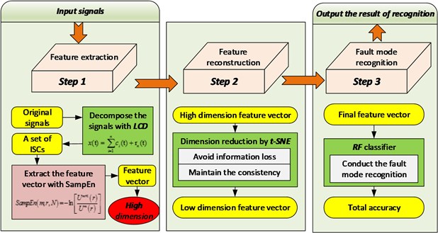
The methodology has three major steps: (1) the LCD is applied to decompose the sensor signals into several ISCs, and the SampEn of each ISC is extracted as the feature vectors; (2) the dimension of the feature vectors is reduced by t-SNE; (3) the feature vectors reconstructed by t-SNE are input into the RF for fault diagnosis. The framework of the methodology is summarized in Fig. 1.
Fig. 1Framework of the proposed methodology
2.1. LCD
The LCD method can self-adaptively decompose a complex signal into a sum of ISCs and a residue, with the assumption that any two ISCs are independent of each other. The decomposition process is shown in Fig. 2. In the figure, the standard deviation (SD) is defined as the criterion to determine whether the decomposition ends. In this study, the value of the SD is set as 0.3. Therefore, when the SD is smaller than 0.3, the decomposition process ends.
The ISCs must meet the following two conditions:
1) In the entire data set, the signal is monotonic between any two adjacent extreme points;
2) Among the whole data set, suppose the extrema of the signal are (, ) ( 1, 2, …, ). Thus, any two adjacent maxima (minima), (, ) and (, ), are connected by a straight line. For the intermediate minima (maxima) , its corresponding point (, ) on this straight line is as follows:
To ensure the smoothness and symmetry of the ISC, the proportions of and remain constant, as described below:
Fig. 2Decomposition process of the LCD
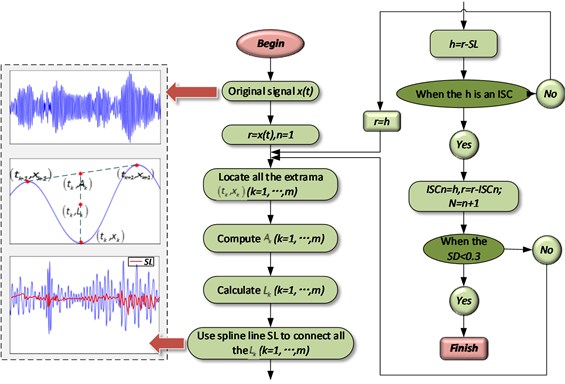
Generally, is set as 0.5; thus, –1. At the time, and are symmetrical about the -axis, thus ensuring the symmetry and smoothness of the ISC component waveform [13].
Based on the definition of the ISC component, a complex signal ( 0) can be decomposed into a sum of ISCs using the LCD method as follows:
1) Suppose the number of extrema of the signal is , and determine all the extrema (, ) ( 1, …, ) of the signal .
2) Compute ( 1, …, ) according to Eq. (1). Based on the following equation, the corresponding ( 1, …, ) can be calculated:
To obtain the values of and , we should extend the boundary of the data; this process can be completed via different methods [14-16]. By extension, two end extrema can be obtained and written as (, ) and (, ) [17]. Using Eq. (1) and Eq. (3), we can obtain and .
3) All the ( 1, …, ) are connected by a cubic spline line , which is defined as the baseline of the LCD.
4) The difference between the data and the baseline is the first component :
5) Separate the first from the initial data:
6) Take the residue as the original signal to be processed. Repeat the above process until the residue is constant, a monotonic function, or a function with no more than twenty extrema.
, …, and the residue are obtained as follows:
where is the th ISC, and is the residue.
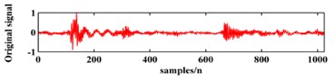
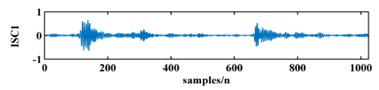
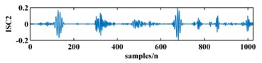
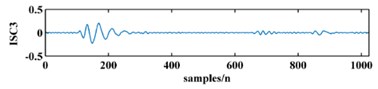
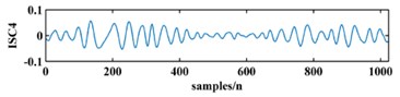
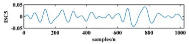
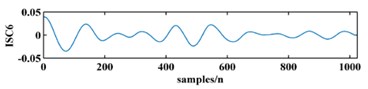
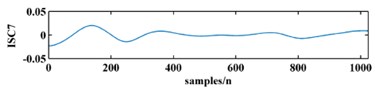
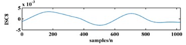
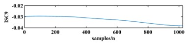
To illustrate the validity of the LCD method, a sample vibration signal of a bearing and its ISCs decomposed by LCD are shown in Fig. 3. The figure shows that the original vibration signal can be effectively decomposed into 9 ISCs.
Fig. 3An original vibration signal of a bearing and its ICSs decomposed by LCD
a)
b)
c)
d)
e)
f)
g)
h)
i)
j)
2.2. SampEn
The LCD method is applied to decompose the original signal into several ISCs with different time scales and characteristics. Next, the SampEn is used to characterize the probability of the new model of the signal, i.e., the change in the values of SampEn when the centrifugal pump works under different conditions can reflect the different fault modes of the centrifugal pump. Thus, the LCD-SampEn can be applied to obtain the feature vector.
The SampEn of a signal of length (, , …, ) is defined as:
where:
And:
In Eq. (8), denotes the number of data points, specifies the pattern length, and is the time delay. In Eq. (4), the symbol is the Heaviside function, given as:
The distance between and (-dimensional pattern vector) is defined as:
And:
The symbol represents a predetermined tolerance value, which is defined as:
where is a constant ( 0), and () represents the standard deviation of the signal. The two patterns and of measurements of the signal are similar if the distance between any pair of corresponding measurements of is less than or equal to [18].
2.3. t-SNE
Stochastic neighbor embedding (SNE) is one of the best performing nonlinear manifold learning algorithms and whose core idea is to maintain the consistency of the neighborhood probability distribution between high-dimensional and low-dimensional space. SNE transfers the traditional Euclidean distance-based similarity measurement to the conditional probability-based similarity measurement: in high-dimensional observation space, the Gaussian distribution is adopted to simulate the similarity relationship between observation samples. The similarity between and is denoted as follows:
where is the bandwidth of the Gaussian kernel function in the observation sample . is the probability of chosen by as its neighbor sample. The parameter obeys a Gaussian distribution, for which the variance is and the mean value is . The probability of and being adjacent to each other is:
In low-dimensional space, SNE continues to adopt the Gaussian distribution to measure the similarity between low-distinction samples. However, two obvious shortcomings exist with SNE: (1) the objective function is too complex to optimize, and the gradient is not as concise as desired; (2) the so-called “crowding problem”; that is, when the data are far apart from each other in high-dimensional space, they must be gathered in the process of mapping to low-dimensional space. In response, t-distributed stochastic neighbor embedding (t-SNE) is introduced to alleviate these problems [19].
To solve the first problem, the characteristic of symmetry is adopted to simplify the objective function and optimize the gradient form, which is referred to as symmetric SNE. According to probability theory, the SNE objective function minimizes the sum of the distances of the conditional probability distribution (high-dimension) and (low-dimension) for the corresponding points. It is equal to the following joint probability distributions of (high-dimension) and (low-dimension):
After adopting a joint probability distribution instead of a conditional probability distribution, the formula is more concise and understandable.
To solve the second problem, the t-distribution function is introduced to alleviate the “crowding problem”. In other words, the t-distribution function is used to measure the similarity of points in low-dimensional space. The joint probability distribution function is as follows:
Here, the t-distribution function (DOF is 1) is applied because of its special advantageous characteristic: is the reciprocal of the distance of points far from each other in low-dimensional space to . In other words, in low-dimensional space, the presentation of the joint probability distribution is insensitive to the distance of points. In addition, in theory, the t-distribution function offers the same performance as the Gaussian function because the t-distribution function can be expressed as the infinity Gaussian function. Thus, the gradient of t-SNE is:
In conclusion, t-SNE focuses on the following:
1) The characteristic of non-similarity is associated with points far from each other. The characteristic of similarity is associated with points close to each other. The t-distribution function is introduced to exert an “exclusion” to process the non-similar points;
2) The application of the t-distribution function makes it easier to optimize.
The t-SNE approach applies a probability density distribution function to measure the similarity and distribution characteristics. Next, t-SNE accomplishes property preservation by minimizing the K-L distance probability density in both high-dimensional and low-dimensional space. The t-distribution function is employed to measure the similarity of points in low-dimensional space, thereby simplifying the gradient form and improves computational speed. Most importantly, the improved processing of the non-similarity points alleviates the “crowding problem”.
2.4. RF
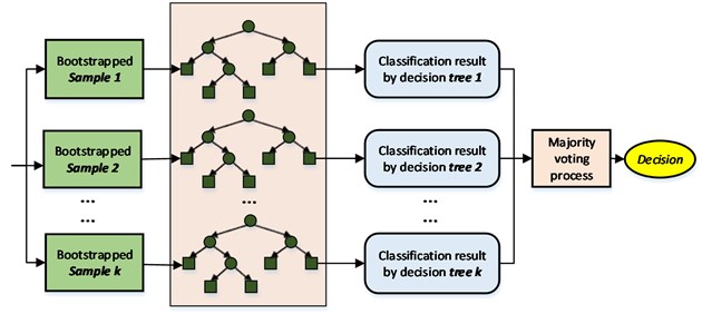
An RF is an ensemble classifier consisting of a collection of tree structured classifiers , 1, ..., where is defined as the independent identically distributed random vectors, and each decision tree casts a unit vote for the most popular class at input X.
A general RF framework is shown in Fig. 4 and is described as follows:
1) By employing bootstrap sampling, samples are selected from the training set, and the sample size of each selected sample is the same as those of the training sets.
2) decision tree models are built for samples, and classification results are obtained by these decision tree models.
3) According to classification results, the final classification result is decided by voting on each record. The RF increases the differences among the classification models by building different training sets; therefore, the extrapolation forecasting ability of the ensemble classification model is enhanced. After times training, a classification model series {, , …, } is obtained; the series is utilized to structure a multi-classification model system. The final classification result of the system is simple majority voting, and the final classification decision is given as Eq. (1):
where is the ensemble classification model, hi is a single decision tree classification model, is the objective output, and is an indicative function. Eq. 14 describes how the final classification is decided by majority voting.
Fig. 4Framework of the RF
3. Case study
As one of the most important rotating parts of machinery, a bearing is also an important source of failure of mechanical equipment. Statistics show that, in the application of rotating machinery, most of the mechanical failure is caused by rolling bearings. In addition, as power components of a hydraulic system, a hydraulic pump, which provides high-pressure hydraulic oil to the entire hydraulic system, is also a typical type of rotating machinery. As a result, bearings and a hydraulic pump are selected to verify the effectiveness of the proposed method.
3.1. Fault diagnosis for a hydraulic pump
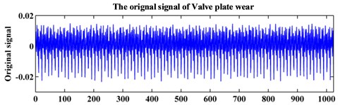
The testing equipment for the axial piston hydraulic pump is shown in Fig. 5. In the experiment, the rotation speed is set at 5280 r/min, and the corresponding spindle frequency is 88 Hz. An accelerograph is installed at the end face of the pump. The sampling frequency is 1 kHz. The collected data contains three fault modes: normal, piston shoes and swashplate wear, and valve plate wear. The original signals of the three fault modes are shown in Fig. 6. Each data sample consists of 1024 points for analysis. Sixty samples are collected for each fault pattern. Thirty samples of each fault pattern are set as the training data, and the other 30 samples are set as the testing data.
Fig. 5A hydraulic pump system
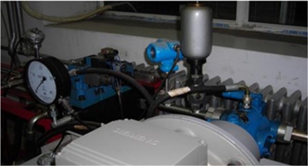
Fig. 6Original signal of the hydraulic pump system
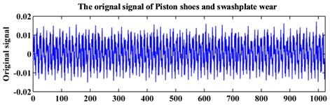
a)
b)
c)
The LCD method is applied to decompose the signals of the normal mode, piston shoes and swashplate wear mode, and valve plate wear mode. To acquire the fault feature vectors, the SampEn is utilized to quantify the ICSs. In this paper, the parameters are set to 2 and 0.2 times the standard deviation of the original signal.
Table 1 shows an example of the feature vectors of each fault mode represented by SampEn of ISCs. As shown in Table 1, because of the high dimension of ISC, the feature vector is usually composed of more than 8 SampEn values, which indicates the dimension of the feature vector is over 8 and makes the recognition of the fault mode difficult.
Table 1Feature vectors represented by SampEn of ISCs for the hydraulic pump
Fault mode | Feature vector | ||||||||
ISC1 | ISC2 | ISC3 | ISC4 | ISC5 | ISC6 | ISC7 | ISC8 | ISC9 | |
Piston shoes and swashplate wear | 0.918 | 1.626 | 1.269 | 0.602 | 0.281 | 0.077 | 0.068 | 0.025 | 0.003 |
Valve plate wear | 1.615 | 0.927 | 0.596 | 0.289 | 0.124 | 0.081 | 0.045 | 0.003 | 0 |
Normal | 1.279 | 1.492 | 1.039 | 0.376 | 0.259 | 0.132 | 0.033 | 0.003 | 0 |
In this paper, t-SNE is used to reduce the dimension of the feature vector. Table 2 shows the results of applying t-SNE to the feature vectors. After using t-SNE, the feature vectors are reconstructed and reduced automatically to 3 dimensions. Through comparison of Table 1 and Table 2, it is obvious that the reconstructed feature vectors exhibit a strong ability of separability after dimension reduction by t-SNE, as shown in Fig. 7. Fig. 7 shows the results of dimension reduction using t-SNE. It provides a desirable input for the classification.
Table 2Reconstructed feature vectors using t-SNE
Fault mode | Reconstructed feature vector | ||
Dimension 1 | Dimension 2 | Dimension 3 | |
Piston shoes and swashplate wear | –84.5229 | 0.3368 | 0.9916 |
Valve plate wear | 0.9960 | 0.0118 | 0.3499 |
Normal | 0.9968 | –0.0352 | –0.7872 |
Fig. 7The feature vector extracted: a) using t-SNE, b) without t-SNE
a)
b)
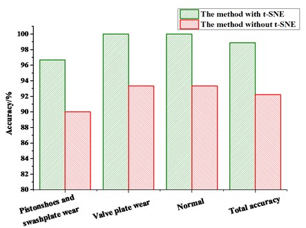
Subsequently, the RF is applied to recognize the fault mode of the hydraulic pump. The results are shown in Table 3 and Fig. 8.
Table 3Comparison of the results
Fault mode | Accuracy [%] | |
The method with t-SNE | The method without t-SNE | |
Piston shoes and swashplate wear | 96.67 | 90.00 |
Valve plate wear | 100.00 | 93.33 |
Normal | 100.00 | 93.33 |
Total accuracy | 98.89 | 92.22 |
From the results diagnosed by the RF, we can see that the proposed method achieves the total accuracy of 98.89 %, in which the accuracy of the normal mode, the valve plate wear mode, and the piston shoes and swashplate wear mode is 96.67 %, 100.00%, and 100.00 %, respectively. However, the method without t-SNE only achieves the accuracy of 92.22 %, and the accuracy of the normal mode, the valve plate wear mode, and the piston shoes and swashplate wear mode is 90.00 %, 93.99 % and 93.33 %, respectively. From the results, it is obvious that after dimension reduction by t-SNE, the accuracy improved greatly. This fully demonstrates the effectiveness of the proposed method.
Fig. 8Comparison results of the diagnostic methods
3.2. Fault diagnosis for a bearing
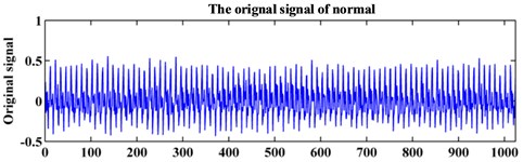
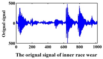
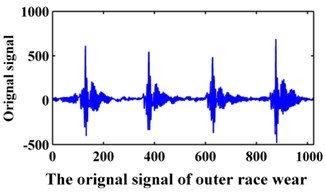
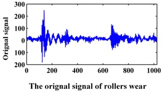
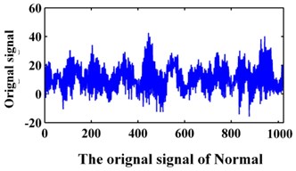
The data of the bearing are from Xi’an Jiaotong University. In the experiment, the sampling frequency is 20 kHz. The data collected contains the following fault modes: normal, bearing inner race wear, bearing outer race wear and bearing rollers wear. The original signals are shown in Fig. 9. A data set of 1024 points for each team is selected for analysis. Then, 100 samples were collected for each fault pattern. Forty samples of each fault pattern are set as the training data, and the other 60 samples are set as the testing data.
Fig. 9Original signals of the bearing
a)
b)
c)
d)
Table 4 presents the obtained SampEn values of these ISCs.
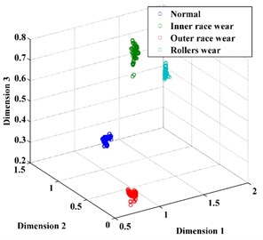
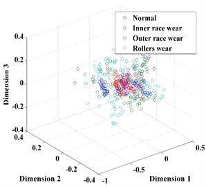
Subsequently, the original features of the datasets are reduced automatically to 3 dimensions by t-SNE. For comparison, the dimension of the feature vector is also reduced by PCA and LPP, as shown in Fig. 10. From Fig. 10, we can conclude that the feature vector reduced by t-SNE exhibits a stronger ability for separability than those reduced by PCA and LPP and thus provides a desirable input for classification.
Table 4Feature vectors represented by SampEn of ISCs for the bearing
Fault mode | Feature vector | ||||||||
ISC1 | ISC 2 | ISC 3 | ISC 4 | ISC 5 | ISC 6 | ISC 7 | ISC 8 | ISC 9 | |
Normal | 1.904 | 1.328 | 0.450 | 0.163 | 0.117 | 0.058 | 0.026 | 0.001 | 5.385∙10-4 |
Inner race wear | 1.049 | 0.545 | 0.847 | 0.484 | 0.264 | 0.132 | 0.048 | 0.018 | 0.002 |
Outer race wear | 0.813 | 0.137 | 0.267 | 0.336 | 0.275 | 0.153 | 0.074 | 0.039 | 0.010 |
Rollers wear | 1.094 | 1.107 | 0.312 | 0.395 | 0.167 | 0.073 | 0.049 | 0.015 | 9.543∙10-4 |
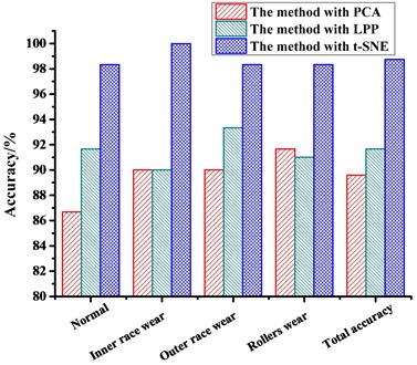
Subsequently, the RF was applied to recognize the states of the hydraulic pump based on the feature vectors obtained by LCD-SampEn and t-SNE. The result is shown in Table 5 and Fig. 11. A comparison of the results obtained by the PCA and LPP methods is also shown in Table 5.
Fig. 10The feature vector extracted using: a) PCA, b) LPP, c) t-SNE
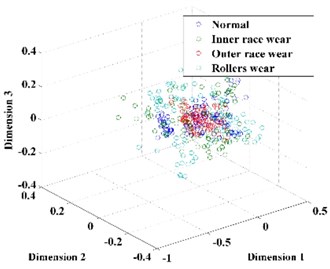
a)
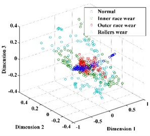
b)
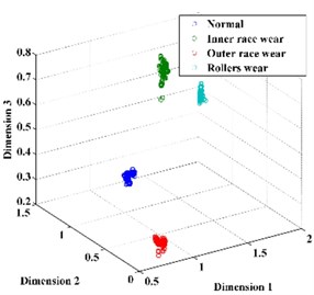
c)
Table 5Comparison of the results of the diagnostic methods
Fault mode | Accuracies of different dimension reduction methods [%] | ||
PCA | LPP | t-SNE | |
Normal | 86.67 | 91.67 | 98.33 |
Inner race wear | 90.00 | 90.00 | 100.00 |
Outer race wear | 90.00 | 93.33 | 98.33 |
Rollers wear | 91.67 | 91. 67 | 98.33 |
Total accuracy | 89.59 | 91.67 | 98.75 |
From the results diagnosed by the RF, we can see that the PCA method shows the worst performance of the three methods; the accuracy rates of the normal mode, the inner race wear mode, the outer race wear mode, and the rollers wear mode are 86.67 %, 90.00 %, 90.00 % and 91.67 %, respectively, and the total accuracy is 89.59 %. The poor results are due to the non-linear nature of the feature, which is not ideal for use with the PCA method, which is a typical linear dimension reduction method. For the LPP method, the accuracy rates of the normal mode, the inner race wear mode, the outer race wear mode, and the rollers wear mode are 91.67 %, 90.00 %, 93.33 % and 91. 67 % respectively, and the average accuracy is 91.67 %. The t-SNE method shows the best performance of the three methods; the accuracy rates of the normal mode, the inner race wear mode, the outer race wear mode, and the rollers wear mode are 98.33 %, 100.00 %, 98.33 % and 98.33 %, respectively, and the total accuracy is 98.75 %. The result verifies the superiority of the t-SNE method in feature dimension reduction and fault diagnosis.
Fig. 11Comparison results of the diagnostic methods
4. Conclusions
In this paper, t-SNE was introduced to the fault diagnostic method to reduce the dimensionality of feature vectors, thereby providing a desirable input for classification and enabling the classifier to achieve a better fault recognition accuracy. The proposed method contains three major steps: first, signal decomposition based on LCD and feature vector extraction based on SampEn; second, dimension reduction based on t-SNE; and third, fault mode recognition based on RF.
In two case studies, the proposed method was applied to two different types of rotating machinery. In the case of the hydraulic pump, the method with t-SNE and the method without t-SNE were studied for comparison, revealing accuracies of 98.89 % and 92.22 %, respectively. The results illustrated fully that, after dimension reduction by the t-SNE, the accuracy of fault diagnosis can be enhanced and the effectiveness of t-SNE is validated. In the second case, we applied three different dimension reduction methods, PCA, LPP and t-SNE, to the fault diagnosis of the bearing. The results demonstrated that the accuracy rate of the t-SNE is 98.75 %, which was the best result among the three methods considered. In both cases, high accuracy of fault diagnosis was achieved, and the results validated the effectiveness and superiority of the proposed method.
References
-
Chen, Li Z., Pan J., Chen G., Zi Y., Yuan J., Chen B., He Z. Wavelet transform based on inner product in fault diagnosis of rotating machinery: a review. Mechanical Systems and Signal Processing, Vol. 70, Issue 71, 2015, p. 1-35.
-
He Z., Guo W., Tang Z. A hybrid fault diagnosis method based on second generation wavelet de-noising and local mean decomposition for rotating machinery. ISA Transactions, 2016, p. 61-211.
-
Zhang, Tang B., Xiao X. Time-frequency interpretation of multi-frequency signal from rotating machinery using an improved Hilbert-Huang transform. Measurement, Vol. 82, 2016, p. 221-239.
-
Lin J., Dou C. The diagnostic line: a novel criterion for condition monitoring of rotating machinery. ISA Transactions, Vol. 59, 2015, p. 232-242.
-
Cempel C., Tabaszewski M. Multidimensional condition monitoring of machines in non-stationary operation. Mechanical Systems and Signal Processing, Vol. 21, Issue 3, 2007, p. 1233-1241.
-
Zheng J., Cheng J., Yang Y. A rolling bearing fault diagnosis approach based on LCD and fuzzy entropy. Mechanism and Machine Theory, Vol. 70, Issue 6, 2013, p. 441-453.
-
Zheng J., Cheng J., Yang Y., Luo S. A rolling bearing fault diagnosis method based on multi-scale fuzzy entropy and variable predictive model-based class discrimination. Mechanism and Machine Theory, Vol. 78, Issue 16, 2014, p. 187-200.
-
Pincus S. M. Approximate entropy as a measure of system complexity. Proceedings of the National Academy of Sciences of the United States of America, Vol. 88, Issue 6, 1991, p. 2297.
-
Richman J. S., Moorman J. R. Physiological time-series analysis using approximate entropy and sample entropy. American Journal of Physiology Heart and Circulatory Physiology, Vol. 278, Issue 6, 2000, p. 2039-2049.
-
Li Y., Xu M., Wei Y., Huang W. A new rolling bearing fault diagnosis method based on multiscale permutation entropy and improved support vector machine based binary tree. Measurement, Vol. 77, 2016, p. 80-94.
-
Bregler C., Omohundro S. M. Nonlinear manifold learning for visual speech recognition. International Conference on Computer Vision, 1995.
-
Laurens V. D., Hinton M. G. Visualizing data using t-SNE. Journal of Machine Learning Research, Vol. 9, Issue 2605, 2008, p. 2579-2605.
-
Liu H., Wang X., Lu C. Rolling bearing fault diagnosis based on LCD-TEO and multifractal detrended fluctuation analysis. Mechanical Systems and Signal Processing, Vol. 60, Issue 61, 2015, p. 273-288.
-
Güneri A. F., Ertay T., Yücel A. An approach based on ANFIS input selection and modeling for supplier selection problem. Expert Systems with Applications, Vol. 38, Issue 12, 2011, p. 14907-14917.
-
Cheng J., Yu D., Yang Y. Application of support vector regression machines to the processing of end effects of Hilbert-Huang transform. Mechanical Systems and Signal Processing, Vol. 21, Issue 3, 2007, p. 1197-1211.
-
Qi K., He Z., Zi Y. Cosine window-based boundary processing method for EMD and its application in rubbing fault diagnosis. Mechanical Systems and Signal Processing, Vol. 21, Issue 7, 2007, p. 2750-2760.
-
Luo S., Cheng J., Ao H. Application of LCD-SVD technique and CRO-SVM method to fault diagnosis for roller bearing. Shock and Vibration, 2015, Vol. 2015, p. 847802.
-
Sokunbi M. O., Cameron G. G., Ahearn T. S., Murray A. D., Staff R. T. Fuzzy approximate entropy analysis of resting state fMRI signal complexity across the adult life span. Medical Engineering and Physics, Vol. 37, Issue 11, 2015, p. 1082-1090.
-
Van Der Maaten, Hinton L. G. Visualizing data using t-SNE. Journal of Machine Learning Research, Vol. 9, 2008, p. 2579-2605.
Cited by
About this article

