Bearing fault diagnosis based on intrinsic time-scale decomposition and improved Support vector machine model

Sheng, Jinlu; Dong, Shaojiang; Liu, Zhu

doi:10.21595/jve.2015.16246

Journal of Vibroengineering

Browse Journal

Submit article

Published: 31 March 2016

Check for updates

Bearing fault diagnosis based on intrinsic time-scale decomposition and improved Support vector machine model

Jinlu Sheng¹

Shaojiang Dong²

Zhu Liu³

¹College of Traffic and Transportation, Chongqing Jiaotong University, Chongqing 400074, China

²School of Mechatronics and Automotive Engineering, Chongqing Jiaotong University, Chongqing 400074, People’s Republic of China

²Key Laboratory of Road Construction Technology and Equipment (Chang’an University), MOE, Xian 710064, People’s Republic of China

³Qingdao Ocean Shipping Mariners College, Qingdao 266071, China

Corresponding Author:

Shaojiang Dong

Cite the article Download PDF

Downloads 1357

CrossRef Citations 5

Abstract

In order to achieve the bearing fault diagnosis so as to ensure the steadiness of rotating machinery. This article proposed a model based on intrinsic time-scale decomposition (ITD) and improved support vector machine method (ISVM), so as to deal with the non-stationary and nonlinear characteristics of bearing vibration signals. Firstly, the feature extraction method intrinsic time-scale decomposition (ITD) is used and the energy entropy are extracted so as to process the vibration signal in this paper. Then, the local tangent space alignment (LTSA) method is introduced to extract the characteristic features and reduce the dimension of the selected entropy features. Finally, the features are used to train the ISVM model as to classify bearings defects. Cases of actual were analyzed. The results validate the effectiveness of the proposed algorithm.

1. Introduction

As vital components in many rotating machinery, the failure of rolling element bearings may cause great economic loss and threaten people’s life. This makes bearing diagnostics a prime research field to improve efficiency and durability of the industrial mechanical systems. Ideal diagnostics should also provide a real-time condition of the components in order to monitor them until the appearance of the first signals of malfunctioning. This could ensure a longer lifetime of the parts than other maintenance techniques, e.g. the preventive maintenance, where components are substituted at given time intervals independently of their actual conditions, with a relevant economic advantage.

However, it is not an easy work to achieve the bearing fault diagnosis. The last two decades, the interest for efficient and robust diagnostics of roller element bearings via condition monitoring approaches as well as advanced signal processing has seen an extremely high increase. Of paramount importance in the diagnostic task are two items: 1) the feature extraction of damage sensitive features from the recorded condition monitoring signals and 2) the pattern recognition approach that leads to fault identification [1, 2].

To extract the fault features, the signal processing tools that usually been applied, such as: time domain analysis, frequency domain analysis and time-frequency domain analysis. Time domain analysis is the simplest, its diagnoses faults mainly by analyzing statistical indicators, such as kurtosis, crest factor and root-mean square, directly extracted from the time series of the vibration signals. Frequency domain methods usually diagnose mechanical faults by observing the fault characteristic frequencies hidden in the vibration signals. Although FFT is the simplest frequency domain analysis method, its frequency resolution is low when there is a small number of sampling points. The time-frequency method is used more commonly. Wavelet transform is the most commonly used time-frequency analysis method and is widely used in feature extraction [3]. However, the selection of the wavelet mother coefficient is difficult, and for different researcher the selected coefficient not unique. So it is necessary to find an effective method to extract the fault-related features hidden in the complex and non-linear bearing vibration signals. The EMD [4] is other tool usually used in time-frequency domain analysis which is suitable for analyzing non-stationary signals. However, the EMD method has the problems of endpoint leak, and the modal aliasing. In this article, the intrinsic time-scale decomposition (ITD) is used to process the collected vibration signal [5, 6] and the ITD Shannon entropy is used to extract the original features from the signal.

However, the ITD energy entropy features remain to be high-dimensional, and excessive redundant information still existed in them. In order to reduce the dimension of the features, the non-linear embedding method local tangent space alignment (LTSA) is used to extract the most useful features as inputs of the bearing running state recognition model [7]. LTSA can achieve the transformation from input space to feature space through the nonlinear mapping method, so it has strong nonlinear dimension reduction ability.

Recognizing condition, in order to identify the work condition of roller bearing further, the SVM is served as a classifier [8, 9]. However, the traditional SVM is not sensitive to the nonlinear feature classification, in recent years, the combination of wavelet theories and SVM has drawn considerable attention owing to its high classification ability for a wide range of applications and better performance than other traditional leaning machines, in this paper, the Morlet kernel is use to construct the new SVM model [10].

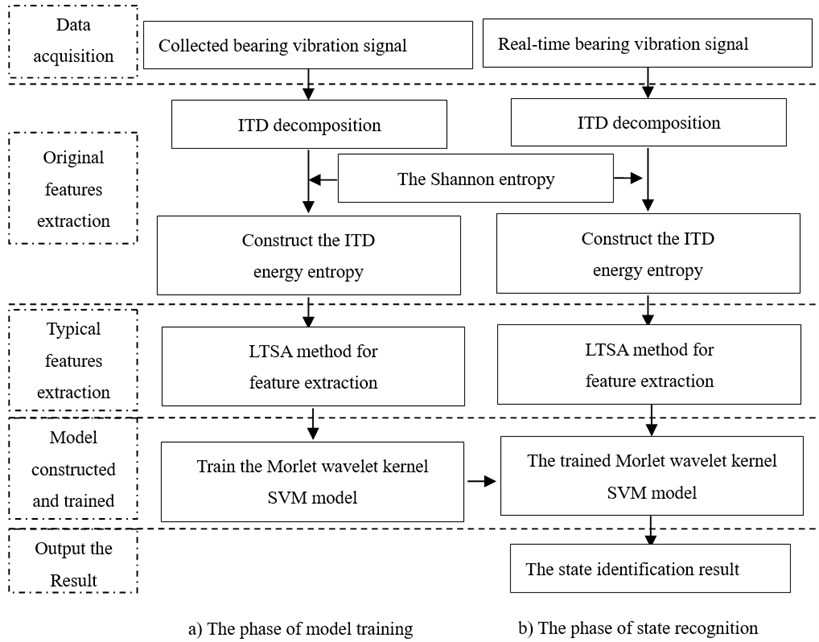
Fig. 1The flowchart of the proposed method

The paper is organized as follows: Section 2 the concept of ITD energy entropy is proposed and the ITD energy entropies of different vibration signals are calculated. In Section 3, the non-linear embedding method LTSA is described. The Morlet wavelet kernel SVM model is presented in Section 4. In Section 5, the degradation state method is applied to roller bearing diagnosis. The conclusion of this paper is given in Section 6.

The flowchart of the proposed method is showed in Fig. 1.

2. Methods of signal processing and Feature extraction

2.1. Signal processing

This section presents a brief discussion on bearing vibration signal processing from ITD. ITD is specifically formulated for application to nonlinear or non-stationary signals of arbitrary origin and obtained from complex systems with underlying dynamics that change on multiple time-scales simultaneously. The ITD overcomes the limitations of EMD listed earlier, as well as those previously mentioned and associated with more classical approaches such as Fourier and wavelets [5].

Given a signal $X_{t}$ , we define an operator $l$ , which extracts a baseline signal from $X_{t}$ in a manner that causes the residual to be a proper rotation. More specifically, $X_{t}$ can be decomposed as:

1

X_{t} = l X_{t} + (1 - l) X_{t} = L_{t} + H_{t},

where $L_{t} = l X_{t}$ is the baseline signal and $H_{t} = (1 - l) X_{t}$ is a proper rotation.

Suppose { $X_{t}$ , $t \geq 0$ } is a real-valued signal, and let { $τ_{k}$ , $k =$ 1, 2, 3, …} denote the local extrema of $X_{t}$ , and for convenience define $τ_{0} = 0$ . In the case of intervals on which $X_{t}$ is constant, but which contain extrema due to neighbouring signal fluctuations, $τ_{k}$ is chosen as the right endpoint of the interval. To simplify notation, let $X_{k}$ and $L_{k}$ denote $X_{τ_{k}}$ and $L_{τ_{k}}$ , respectively.

Suppose that $L_{t}$ and $H_{t}$ have been defined on [0, $τ_{k}$ ] and that $X_{t}$ is available for $t \in [0, τ_{k + 2}]$ . We can then define a (piece-wise linear) baseline-extracting operator $l$ , on the interval ( $τ_{k}$ , $τ_{k + 1}$ ] between successive extrema as follows:

2

L_{t} = l X_{t} = L_{k} + (\frac{L_{k + 1} - L_{k}}{X_{k + 1} - X_{k}}) (X_{t} - X_{k}), t \in (τ_{k}, τ_{k + 1}],

where:

3

L_{k + 1} = α [X_{k} + (\frac{τ_{k + 1} - τ_{k}}{τ_{k + 2} - τ_{k}}) (X_{k + 2} - X_{k})] + (1 - α) X_{k + 1},

and 0 $< α <$ 1 is typically fixed with $α =$ 1/2. We construct the baseline signal $L_{t}$ , in this manner in order to maintain the monotonicity of $X_{t}$ between extrema, while at the same time remaining inside an envelope generated by some wave riding atop this baseline. The extrema are interpreted as evidence of some proper rotation, riding wave to be extracted. The baseline is constructed as a linearly transformed contraction of the original signal in order to make the residual function monotonic between extrema, a necessity for proper rotations. The approach also enables information ‘intrinsic’ to the original signal to be passed down to the baseline and residual components. We found that other attempts at baseline construction that were not based on use of the input signal, inevitably failed to produce proper rotation residuals.

After defining the baseline signal according to Eqs. (2) and (3), we are able to define the residual, proper-rotation-extracting operator $ℏ$ , as:

4

ℏ X_{t} = (1 - l) X_{t} = H_{t} = X_{t} - L_{t} .

Through the decomposition of the original signal, the intrinsic scale component (ISC) can be acquired, which represents different frequency components of original signal. Which can be represents as:

5

x (t) = \sum_{p = 1}^{n} I S C_{p} (t) + r_{n} (t) .

2.2. Feature extraction

Once the $n$ ISCs and a residue $r_{n} (t)$ are obtained, where the energy of the $n$ ISCs is $E_{1},$ $E_{2}$ , …, $E_{n}$ can be calculated respectively; then, due to the orthogonality of the ITD decomposition, the sum of the energy of the $n$ ISCs should be equal to the total energy of the original signal when the residue $r_{n} (t)$ is ignored. As the ISCs $c_{1} (t),$ $c_{2} (t)$ , …, $c_{n} (t)$ include different frequency components, $E = {E_{1}$ , $E_{2}$ , …, $E_{n}}$ forms an energy distribution in the frequency domain of roller bearing vibration signal, and then the corresponding ITD energy entropy is designated as:

6

H_{e n t r o p y} = - \sum_{i = 1}^{n} p_{i} l o g p_{i},

where $p_{i} = E_{i} / E$ is the percent of the energy of $c_{i} (t)$ in the whole signal energy ( $E = \sum_{i = 1}^{n} E_{i}$ ).

3. Basic concepts of Local tangent space alignment

The basic idea of LTSA is to use the tangent space of sample points to represent the geometry of the local character. Then these local manifold structures of space are lined up to construct the global coordinates. Given a data set $X =$ [ $x_{1}$ , $x_{2}$ , …, $x_{N}$ ], $x_{i} \in R^{m}$ , a mainstream shape of $d$ -dimension ( $m > d$ ) is extracted. The LTSA feature extraction algorithm is as follows [11]:

1) Extract local information: for each $x_{i}$ , $i =$ 1, 2, …, $N$ , used the Euclidean distance to determine a set $x_{i} =$ [ $x_{i, 1}$ , $x_{i, 2}$ , …, $x_{i, k_{i}}$ ] of its neighborhood adjacent points ( $k$ nearest neighbors, for example).

2) Local linear fitting: In the neighborhood of data points $x_{i}$ , a set of orthogonal basis $Q_{i}$ can be selected to construct the $d$ -dimension neighborhood space of $x_{i}$ and the orthogonal projection of each point $x_{i, j}$ ( $j =$ 1, 2, …, $N$ ) can be calculated to the tangent space of $θ_{j}^{(i)} = Q_{i}^{T} (x_{i, j} - {\bar{x}}_{i}$ ). ${\bar{x}}_{i}$ is the mean data for the neighborhood. The orthogonal projection in the tangent space of neighborhood data of $x_{i}$ is composed of local coordinate $Θ_{i} =$ [ $θ_{(i), 1},$ $θ_{(i), 2}$ , …, $θ_{(i), k_{i}}$ ] that describes the most important information of the geometry of the $x_{i}$ .

3) Global order of the Local coordinates: supposing the global coordinates of $x_{i}$ converted by the $Θ_{i}$ is $T_{i} =$ [ $t_{i 1}$ , $t_{i 2}$ , …, $t_{i k_{i}}$ ], then the error is:

7

E_{i} = T_{i} [I - (1 / k) e] - L_{i} Θ_{i},

where the $I$ is the identity matrix; the $e$ is the unit vector; the $k$ is the points number of the neighborhood; The $L_{i}$ is the transformation matrix. In order to minimize the error, the $T_{i}$ and $L_{i}$ should be found, then:

8

L_{i} = T_{i} (I - (1 / k) e) Θ_{i}^{*},

9

E_{i} = T_{i} (I - (1 / k) e) (I - Θ_{i}^{*} Θ_{i}),

where: the $Θ_{i}^{*}$ is the Moor-Penrose generalized inverse of $Θ_{i}$ . Supposing the:

10

B = P W W^{T} P^{T} .

Let $P =$ [ $P_{1}$ , $P_{2}$ , …, $P_{N}$ ], $T P_{i} = T_{i}$ , $P_{i}$ is a selected matrix from 0-1, the $T$ are global coordinates, their weight matrix:

11

W = d i a g (W_{1}, W_{2}, \dots, W_{N}),

12

W_{i} = (I - (1 / k) e) (I - Θ_{i}^{*} Θ_{i}) .

The constraints is:

13

T T^{T} = I_{d} .

4) Extract of the low-dimensional manifolds feature: Since the $e$ is the eigenvalue of matrix $B$ , so the corresponding minimum eigenvectors matrix is composed of eigenvalue. Section 2 to section $d + 1$ of matrix $B$ make of the $T$ . $T$ is the global coordinate mapping in the Mainstream form of low-dimensional transformed from the non-linear high-dimensional data set of $X$ .

4. The Morlet wavelet kernel SVM model

The support vector’s kernel function can be described as not only the product of point, such as $k (x, x') = k (〈x \cdot x'〉)$ , but also the horizontal floating function, such as $k (x, x') = k (〈x \cdot x'〉)$ , In fact, if a function satisfies the condition of Mercer’s Theorem, it is the allowable support vector’s kernel function. A specific Mercer’s Theorem description can be found in literature [10].

According to Mercer’s Theorem, the number of wavelet kernel functions which can be shown by existent functions is few. Now, an existent wavelet kernel is given, the Morlet wavelet kernel. It can prove that this function can satisfy the condition of allowable support vector’s kernel function. The Morlet wavelet function is defined as follows:

14

ψ (x) = c o s (w_{o} x) e^{- \frac{x^{2}}{2}} .

The Morlet wavelet kernel function is defined as follows:

15

k (x, x') = k (x - x') = \prod_{i = 1}^{d} ψ (\frac{x_{i} - x_{i}^{'}}{a_{i}}) = \prod_{i = 1}^{d} \cos [w_{o} (\frac{x_{i} - x_{i}^{'}}{a_{i}})] e^{[- \frac{(x_{i} - x_{i}^{'})^{2}}{2 {a_{i}}^{2}}]} .

Then, the Morlet wavelet kernel function is being used as the support vector’s kernel function, the SVM is defined as:

16

f (x) = s g n \{\sum_{i = 1}^{n} a_{i} y_{i} \prod_{j = 1}^{d} \cos [w_{o} (\frac{x_{j} - x_{j}^{'}}{a_{j}})] \times e^{[- \frac{(x_{j} - x_{j}^{'})^{2}}{2 {a_{j}}^{2}}]} + b\} .

Through the Eqs. (15) and (16), the Morlet wavelet kernel SVM is constructed, and the new constructed SVM which is effective in classification is used the achieve bearing fault diagnosis.

The method consists of 3 procedures sequentially: data processing and features extracting, merge of the original features, constructing-training ISVM model for fault diagnosis. The role of each procedure is explained as follows:

Step 1. Data processing and features extraction. The ITD signal processing methods are used to extract the original features from the collected mass vibration data.

Step 2. Merge of the original features. The LTSA method is used to extract the typical features and reduce the dimension of the features. The extracted features are used for training the ISVM model.

Step 3. Construct the ISVM model. The ISVM model is constructed. The rotating machine fault diagnosis is achieved.

5. Validation

5.1. Case 1

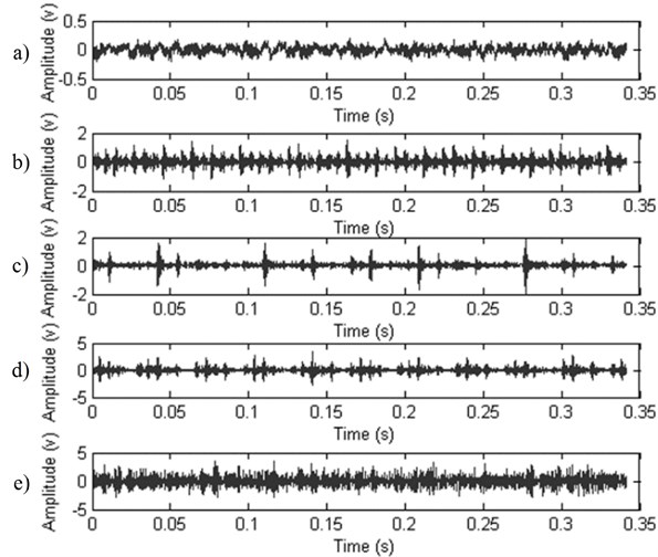
In order to verify the effectiveness of the proposed method, the bearing running state data sets of the normal state and several fault states were analyzed. The proposed method was applied to bearing fault signals obtained from the Case Western Reserve University [12]. The bearing type in the experiments is SKF 6205-2RS JEM. Experiments were conducted by using a 2 hp reliance electric motor. Bearings were seeded with faults by using electro-discharge machining. The test is to simulate the bearing normal running state and fault running states, with fault depth of 0.18 mm, 0.36 mm, 0.53 mm and 0.71 mm at the inner raceway, outer raceway and the ball to reflect the deteriorating state of the bearing; the inner raceway fault signals were chosen in this case. Data was collected at the rate of 12,000 samples per second. 4096 data points were selected to analyze. 50 groups of test data of each fault states were selected, with 20 groups for training, the other 30 groups for testing. The collected vibration signals of normal state and inner-race four different fault depths are shown in Fig. 2.

Fig. 2The collected vibration signals of normal state and inner-race four different fault depths

Next, the ITD decomposition was used to decompose each group of signals into ISCs, and Shannon entropy was used to extract the features. A group of inner-race entropy of Fig. 2 is obtained, the 0.71 mm inner raceway fault ISCs (decomposed in 5 ISCs) decomposed by ITD as shown in Fig. 3.

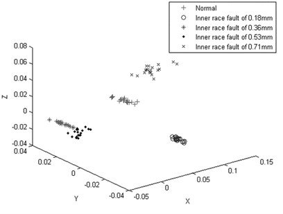
Then, normalize the 20 groups of entropy values, and input them into the LTSA to reduce the dimension. In order to compare the dimension reduction and redundant treatment effect of LTSA, the principle component analysis (PCA) [13], and the Kernel based principle component analysis (KPCA) [14] method is used to reduce the dimension. The results are shown in Figs. 4, 5, and 6. To be comparable, the dimensions of PCA, KPCA and LTSA, are set to 5, so the input dimension of ISVM is 5 and the neighborhood number is set to 10.

By comparing Figs. 4, 5, and 6, the results show that the PCA-based data dimension reduction method can’t effectively separate the high dimension features, and there is still serious aliasing, which will affect the accuracy of the ISVM state recognition effect. The KPCA-based data dimension reduction method works better than the PCA methods, however, there still have some data mixed together. The LTSA-based data dimension reduction method can effectively separate the features of different running states with high calculation accuracy and a higher computational efficiency than the PCA and KPCA methods, which conform more to the actual project requirement. Thus, in the study, the LTSA method is selected.

Fig. 3The 0.71 mm inner raceway fault ISCs (decomposed in 5 ISCs) decomposed by ITD

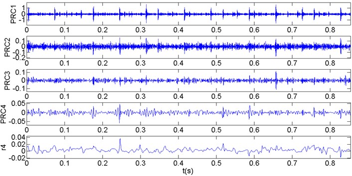
Fig. 4The feature processed effect by the PCA

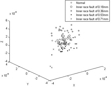
Fig. 5The feature processed effect by the KPCA

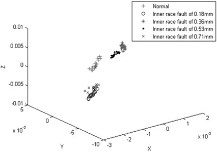
Fig. 6The feature processed effect by the LTSA

After dimension reduction with the LTSA, the extracted features are input into the ISVM (the wavelet of Morlet with $w_{0}$ set to 5, $a_{j}$ equal to $a$ set to 0.3) to train the model so as to recognize the states. In order to compare the identifying effect with and without manifold learning method, the following comparisons are done:

Use ITD Shannon entropy to extract the features and directly input the extract features into the ISV, without the KPCA dimension reduction process.

1) Use ITD Shannon entropy to extract the features and process the extracted features by PCA to reduce the dimension, then input the features into the ISVM.

2) Use ITD Shannon entropy to extract the features and process the extracted features by KPCA to reduce the dimension, then input the features into the ISVM.

3) The method proposed in this article.

The comparison results are shown in Table 1.

Table 1The states recognition rate of three different methods (recognition rate η %)

States recognition methods	Normal state	0.18 mm fault depth	0.36 mm fault depth	0.53 mm fault depth	0.71 mm fault depth
Without LTSA dimension reduction	68	64	80	85	80
Use the PCA method dimension reduction	78	67	90	84	92
Use the KPCA method dimension reduction	96	92	98	97	99
Use the LTSA method dimension reduction	100	100	100	100	100

Table 1 showing that after the LTSA-based dimension reduction method and features extraction, the accuracy of states recognition improved significantly, much higher than the other algorithms. Therefore, the use of LTSA for dimension reduction in this research is necessary and valuable.

In order to further verify the identification accuracy of the proposed method, the features extracted by LTSA are input into the BP neural network (with the learning rate of the neural network is 0.01; The iteration number is 2000; the training error is 0.001; The hidden number $n =$ 15). the RBF SVM (with penalty factor $C$ set to 100, nuclear parameter $γ$ set to 0.1) and the proposed method. The comparison results are shown in Table 2.

Table 2The recognition rate of BPNN, SVM and the ISVM

Model type	Recognition rate $η$ / %
Model type	Normal state	0.18 mm fault depth	0.36 mm fault depth	0.53 mm fault depth	0.71 mm fault depth
BPNN	95	96	94	93	96
SVM	95	93	95	96	95
ISVM	100	100	100	100	100

Table 2 shows that the ISVM can better identify and approach the sensitive features than the SVM and BPNN because of the Morlet kernel wavelet is used. Thus the choice of ISVM to determine the bearing running states can effectively improve recognition accuracy.

Next, a comparison about the training and test time loss of different methods is implemented:

1) The vibration data processed by ITD Shannon entropy and the extract features are direct input into the ISVM, without the LTSA dimension reduction.

2) The vibration data processed by ITD Shannon entropy and the features are processed by LTSA to reduce the dimension; then the extracted features are input into the SVM.

3) The proposed method in this research.

The comparison results are shown in Table 3.

In Table 3, after the dimension reduction, the recognition speed of ISVM improved significantly. The time loss of the proposed method is the shortest. The reason is that the LTSA can extract the typical features and the Morlet kernel can improve the SVM model so as to quickly get the cluster centers. The result validates the proposed method and can effectively recognize the bearing fault.

Table 3The time loss of three different methods

Methods	Without LTSA dimension reduction	SVM method	The proposed method
Time/s	101	73	60

5.2. Case 2

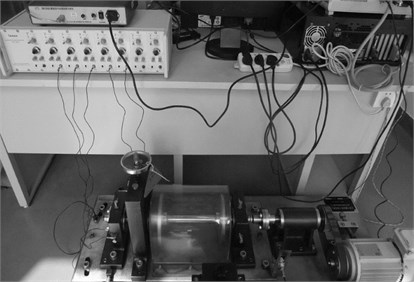
After validating the efficacy of the proposed method, the method is used on another case. The test rig is shown in Fig. 7.

Fig. 7The test rig

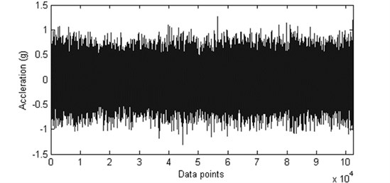
The bearings are hosted on the shaft; the shaft is driven by AC motor. The rotation speed is kept at 1000 rpm; a radial load of 3 kg is added to the bearing. The data sampling rate is 25600 Hz and the data length is 102400 collected points, as shown in Fig. 8. Every 2 hours, the vibration data is collected once. The bearing is run for one year. Then a set of data from each of the 2 months is selected; the data sets are used to test whether or not the proposed method can identify the bearing running state. 4096 data points are selected to analyze, and 60 groups of collected data of different faults are obtained, with 30 groups for training and the other 30 groups for testing.

Fig. 8The collected vibration data

Next, the ITD decomposition was used to decompose each group of signals into ISCs, and Shannon entropy was used to extract the features. A group of features of different fault conditions are obtained, as shown in Table 4 (not normalized beforehand).

Then, the 30 groups’ entropy values are normalized and input into the LTSA in order to reduce the dimension and extract the typical features; the extracted features are input into the improved SVM. The recognize results are shown in Table 5.

Table 5 shows that, although the actual bearing running state is very complex, the proposed method yields a high recognize accuracy. The results confirm that the proposed method can recognize the bearing running states effectively.

Table 4A group of ITD energy entropy of different running states of the actual signal

Running states	$H_{1}$	$H_{2}$	$H_{3}$	$H_{4}$	$H_{5}$
Normal state	1.2157	1.2516	1.2191	1.2012	1.2143
Running for 2 months	1.0324	1. 0451	1.1352	1.2466	1.3910
Running for 4 months	0.6806	0.8996	0.8997	1.0966	0.9959
Running for 6 months	0.9923	0.8769	0.8989	0.8343	0.8675
Running for 8 months	0.6231	0.5338	0.6562	0.6897	0.7122
Running for 10 months	0.7003	0.7085	0.7891	0.7456	0.8321
Running for 12 months	0.7349	0.7893	0.8789	0.7431	0.8324

Table 5The states recognition rate of different states based on the proposed method (recognition rate η %)

Running states	Recognition rate $η$ %
Normal state	100
Running for 2 months	95
Running for 4 months	92
Running for 6 months	93
Running for 8 months	95
Running for 10 months	99
Running for 12 months	100

6. Conclusion

Firstly, this research used the ITD Shannon entropy method to extract the original features from the vibration signals. The LTSA was used to reduce the dimension and data redundancy of the entropy features. Through those methods, the typical features could be extracted effectively.

Then, in order to more accurately identify the bearing running state, the Morlet kernel wavelet model is used to improve and construct the SVM, so as to improve the recognition accuracy of SVM effectively.

Thirdly, through different comparisons we can see that the proposed method makes good use of the advantage of all parts and together to obtain better recognition accuracy and efficiency.

Finally, through the tested signals in the research, the results show the significant efficacy of the proposed method in identifying the bearing faults.

References

George G., Petros K., Theodoros L. Rolling element bearings diagnostics using the symbolic aggregate approximation. Mechanical Systems and Signal Processing, Vol. 60, 2015, p. 229-242.

Publisher
Yan R., Gao R. X., Chen X. Wavelets for fault diagnosis of rotary machines: a review with applications. Signal Processing, Vol. 96, 2014, p. 1-15.

Publisher
Du S. C., Huang D. L. Recognition of concurrent control chart patterns using wavelet transform decomposition and multiclass support vector machines. Computers and Industrial Engineering, Vol. 66, 2013, p. 683-695.

Publisher
Tang B. P., Dong S. J. Method for eliminating mode mixing of empirical mode decomposition based on the revised blind source separation. Signal Processing, Vol. 92, 2012, p. 248-258.

Publisher
Yang Y., Pan H. Y., Ma L. A roller bearing fault diagnosis method based on the improved ITD and RRVPMCD. Measurement, Vol. 55, 2014, p. 255-264.

Publisher
Guo Z. X., Xie L., Ye T. H. Online detection of time-variant oscillations based on improved ITD. Control Engineering Practice, Vol. 32, 2014, p. 64-72.

Publisher
Dong S. J., Chen L. L., Tang B. P. Rotating machine fault diagnosis based on optimal morphological filter and local tangent space alignment. Shock and Vibration, Vol. 9, 2015, p. 1-9.

Publisher
Dong S. J., Luo T. H. Bearing degradation process prediction based on the PCA and optimized LS-SVM model. Measurement, Vol. 46, 2013, p. 3143-3152.

Publisher
Du S. C., Lv J. Minimal Euclidean distance chart based on support vector regression for monitoring mean shifts of auto-correlated processes. International Journal of Production Economics, Vol. 141, 2013, p. 377-387.

Publisher
Gryllias K. C., Antoniadis I. A. A support vector machine approach based on physical model training for rolling element bearing fault detection in industrial environments. Engineering Applications of Artificial Intelligence, Vol. 25, 2012, p. 326-344.

Publisher
Zhang T. H., Yang J., Zhao D. L., Ge X. L. Linear local tangent space alignment and application to face recognition. Neurocomputing, Vol. 70, 2007, p. 1547-1553.

Publisher
Case Western Reserve University Bearing Data Center. http://www.eecs.cwru.edu/laboratory/bearing, 2009.

Search CrossRef
Malhi A., Gao R. X. PCA-based feature selection scheme for machine defect classification. IEEE Transactions on Instrumentation and Measurement, Vol. 53, 2004, p. 1517-1525.

Publisher
Dong S. J., Sun D. H., Tang B. P. Bearing degradation state recognition based on kernel PCA and wavelet kernel SVM. Proceedings of the Institution of Mechanical Engineers, Part C: Journal of Mechanical Engineering Science, Vol. 9, 2015, p. 1-8.

Search CrossRef

Cited by

Bearing fault diagnosis based on optimal Morlet wavelet filter and Teager-Kaiser energy operator

Hocine Bendjama

(2022)

Criteria for optimizing kernel methods in fault monitoring process: A survey

José M. Bernal-de-Lázaro | Carlos Cruz-Corona | Antônio J. Silva-Neto | Orestes Llanes-Santiago

(2022)

A Deep Convolutional Generative Adversarial Networks-Based Method for Defect Detection in Small Sample Industrial Parts Images

(2022)

Fault diagnosis for the gearbox of wind turbine combining ensemble intrinsic time-scale decomposition with Wigner bi-spectrum entropy

Aijun Hu | Ling Xiang | Nan Gao

(2017)

Curve similarity recognition based rolling bearing degradation state estimation and lifetime prediction

Lipin Zhang | Chen Lu | Laifa Tao

(2016)

About this article

Received

04 August 2015

Accepted

13 December 2015

Published

31 March 2016

SUBJECTS

Fault diagnosis based on vibration signal analysis

DOI

https://doi.org/10.21595/jve.2015.16246

Keywords

intrinsic time-scale decomposition

local tangent space alignment

improved support vector machine method

bearing

Acknowledgements

This research is supported by the National Natural Science Foundation of China (No. 51405047), Scientific Research Fund of Chongqing Municipal Education Commission (No. KJ1500529). Science Application Research Project of COSCO, China (Grant No. 2010-1-H-001). Chongqing Postdoctoral Science Foundation funded Project (No. xm2015001). Key Laboratory of Road Construction Technology and Equipment (Chang’an University), MOE (No. 2014SZS11-K02). Natural Science Foundation Project of CQ cstc2013jcyjA70012. China Postdoctoral Science Foundation funded this research, Project No. 2014M552316. The authors are grateful to the anonymous reviewers for their helpful comments and constructive suggestions.

This is an open access article distributed under the Creative Commons Attribution License, which permits unrestricted use, distribution, and reproduction in any medium, provided the original work is properly cited.