Abstract
The high dimensionality data originating from rolling bearing measuring signals with non-linearity and low signal to noise ratio often contains too much disturbance like interference and redundancy for accurate condition identification. A novel manifold learning named Local coordinate weight reconstruction (LCWR) is proposed to remove such disturbance. Due to the different contribution of samples to their manifold structure, weight value is used for the contribution difference. By reconstructing local low-dimensional coordinates according to its weight function about geodesic distance in neighborhood, LCWR targets to reduce reconstruction error, preserve intrinsic structure of the high dimensionality data, eradicate disturbance and extract sensitive features as global low-dimensional coordinates. The experimental results show that the intraclass aggregation and interclass differences of global low-dimensional coordinates extracted via LCWR are better than those of local tangent space alignment (LTSA), locally linear embedding (LLE) and principal component analysis (PCA). The accuracy reaches the highest 96.43 % using SVM to identify LCWR based global low-dimensional coordinates, and its effectiveness is testified in diagnosis of rolling bearing fault.
Highlights
- A manifold learning named Local coordinate weight reconstruction (LCWR) is proposed for nonlinear dimensionality reduction.
- LCWR targets to eradicate disturbance and extract sensitive features from the high dimensionality data.
- The intraclass aggregation and interclass differences of global low-dimensional coordinates via LCWR are better than other methods.
- The accuracy reaches the highest 96.43% and testifies the effectiveness of LCWR in diagnosis of rolling bearing fault.
1. Introduction
Rolling bearing plays a key role in rotating machinery. It is necessary to monitor rolling bearing condition and identify its fault to avoid accident [1-3]. The state information of rolling bearing is usually described with high dimensionality data consisting of multiple characteristics in time and frequency domain [4-6], which contains redundancy and interference, and exists nonlinearity. Therefore, several works have been explored to remove such disturbance and obtain low-dimensional sensitivity features for better accuracy and efficiency of rolling bearing fault [7, 8].
As a type of classic manifold learning for dimensionality reduction [9, 10], local tangent space alignment (LTSA) completing nonlinear dimensionality reduction through finding out neighborhoods of high dimensionality samples, carrying out local dimensionality reduction, and realigning all neighborhoods’ low-dimensional coordinates to construct global low-dimensional coordinates [11], recently has been used for fault diagnosis besides its earlier successful applications to image processing, data mining, machine learning, etc. [12, 13]. For instance, Zhang et al. proposed supervised locally tangent space alignment (S-LTSA) to optimize the neighborhood selection of LTSA based on the training samples’ categories, so that the neighborhood includes the same samples as possible to accurately reflect the local structures of different types of bearing fault signals [14]. Li et al. improved the accuracy of bearing fault diagnosis using LLTSA dimensionality reduction [15]. Kumar A and Kumar R utilized Linear Local Tangent Space Alignment (LLTSA) to suppress noise and retain characteristic defect frequencies of rolling bearing with inner and ball fault [16]. Su et al. proposed orthogonal supervised linear local tangent space alignment (OSLLTSA) to make the neighborhood selection of LLTSA better by introducing sample’s label information, which removed interference and redundancy in high dimensionality fault data and extracted low-dimensional sensitivity fault features [17]. Wang et al. proposed supervised incremental local tangent space alignment (SILTSA) through embedding supervised learning into the incremental local tangent space alignment to extract bearing fault characteristics, process new samples and classify [18]. Su et al. stated supervised extended local tangent space alignment (SE-LTSA) to enhance intraclass aggregation and interclass differences of nonlinear high dimensionality samples by defining distance between samples and optimizing neighborhood choice based on class label [19]. In summary, the current interests focused on neighborhood optimization options and local tangent space estimation of LTSA for dimensionality reduction and low-dimensional sensitivity fault characteristics extraction.
Different from above methods, local coordinate weight reconstruction (LCWR) manifold learning is proposed to reconstruct local coordinates by weight coefficient, so as to extract global low-dimensional sensitivity features for improving fault diagnosis capability of rolling bearing. The following is as below: Section 2 proposes LCWR for coordinate reconstruction, Section 3 validates LCWR and Section 4 is conclusions.
2. LCWR
LCWR has two major tasks. First, the projection coordinates of k nearest neighbors of each sample on the tangent space of the neighborhood are calculated to build the local low-dimensional manifold using LTSA. Next, the global low-dimensional coordinates are obtained by aligning the low-dimensional coordinates of all neighborhoods according to weight coefficient, which is a main innovation of LCWR.
2.1. Local coordinate computation
Let sample matrix , is the number of sample dimensions and is the number of samples. Sample and its nearest samples (including ) constitute local neighborhood matrix , each neighborhood exists a local tangent space consisting of standard orthogonal basis vectors, and is the projection of onto . For the main geometric structure information within neighborhood, minimize the sum of square of distance between and :
where is a mean matrix of , is a unit column matrix of length , and is a by unit matrix.
Apply singular value decomposition to :
, , are computed as below:
where is a left singular vector set, is a right singular vector set, is a singular value diagonal matrix, is a diagonal matrix with maximum singular values in descending order, is the corresponding left singular vector set and is right singular vector set.
Thus, holds the most important geometric structure information in .
2.2. Global coordinate construction
Suppose is the local low-dimensional coordinate of . Build the affine transformation between and :
The local reconstruction error is written as:
where is a local affine matrix, is a mean matrix of , is a local reconstruction error matrix.
However, owing to the different contribution of samples to their manifold structure, a novel LCWR based on weight coefficient is proposed to reduce permutation error and reconstruct local coordinates more accurately. According to LCWR, the closer a sample is to its manifold, the larger its weight coefficient is. Likewise, the farther a sample is from its manifold, the smaller its weight coefficient is. So an exponential function of geodesic distance between a sample and the center point of its neighborhood, reflecting the proximity to its manifold structure, is defined as weight coefficient, namely:
where denotes the weight coefficients of the th nearest neighbor in , and denote the geodesic distance from to the center of and the mean square error of respectively, and is adjustment parameter.
Then is rewritten as:
where is a weight coefficient matrix, .
Fix and minimize to preserve as much local information as possible, namely:
where , .
Substitute Eq. (9) into Eq. (7) and obtain :
where .
Minimize the sum of all neighborhoods reconstruction errors to obtain the global low-dimensional coordinate :
where is the global low-dimensional coordinate of , , is a selection matrix, , is the subscript of nearest neighbors of .
It is equal to solve differential equation:
where .
Therefore, the optimal solution of is composed of eigenvectors corresponding to the 2nd to the ()th smallest eigenvalues of . or is an orthogonal global low-dimensional coordinate mapping matrix of nonlinear manifold in , where is an eigenvector corresponding to the th eigenvalue of .
LCWR is summarized as follows:
(1) Look for neighborhood. Local neighborhood of each sample () is found by k nearest neighbors.
(2) Extract local coordinates. Projection matrix and local low-dimensional coordinate matrix of each neighborhood are obtained according to Eq. (2) and Eq. (3), respectively.
(3) Construct global coordinates. Global low-dimensional coordinate matrix is conducted from reconstruction by weight coefficient matrix and expressed as Eq. (14).
The flow chart of LCWR is shown in Fig. 1.
3. Verification and analysis
Experimental data is from the bearing data center of Case Western Reserve University. Four types of bearing sates under speed of 1750 rpm and load of 1470 W, i.e. healthy state, outer race fault, inner race fault and ball fault with defective size of 0.3556 mm are considered. There are 48 samples for each state and total 192 samples for all states. Each sample acquired at 48 kHz includes 2048 points in length.
3.1. High-dimensional feature construction
As shown in Table 1, 12 time-domain statistical indicators and 8 frequency-domain statistical indicators are selected to constitute a 20-dimensional sample to characterize the bearing state. An original sample signal is decomposed into eight sub-band signals by three-layer db8 wavelet packet decomposition, and the ratio of the energy of each sub-band to the total energy of all sub-bands is taken as the frequency domain indicator. That is, , , is the energy of sub-band signals. Thus, a high-dimensional feature matrix is created.
Fig. 1Procedure of LCWR
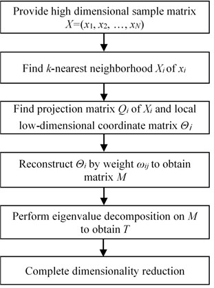
Fig. 2LCWR based fault diagnosis
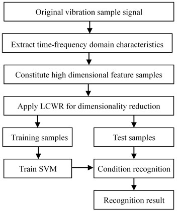
Table 1Basic size and style requirements
Dimension | Description |
1 | Standard deviation |
2 | Variance |
3 | Skewness |
4 | Kurtosis |
5 | Range |
6 | Minimum |
7 | Maximum |
8 | Sum |
9 | Root mean square |
10 | Median |
11 | Mean |
12 | Crest factor |
13-20 | Energy ratio |
3.2. Low-dimensional feature extraction
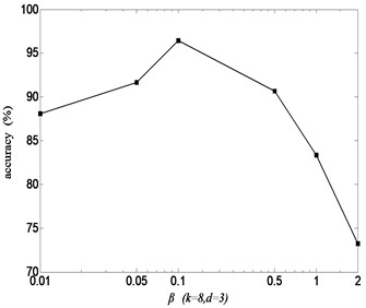
According to Fig. 2, some of the low-dimensional feature samples extracted by LCWR are used as training samples to train support vector machine (SVM) while the others as test samples to be recognized by trained SVM. When using LCWR to extract bearing state characteristics, three parameters such as neighbor number , dimension and adjustment parameter need to be optimized. Because the recognition rate can be regarded as a function of three parameters , and , these parameters interact to determine the recognition rate. By changing these parameters in a certain range and the corresponding recognition rate obtained, it is proved that there exist optimization values of parameters with the peak recognition rate. The trend of recognition rate with respect to a single parameter variable while the other two parameters fixed is shown in Fig. 3-5, respectively. Because of different parameters, the trend of recognition rate is also different from each other.
From the recognition rate about the nearest neighbor number in Fig. 3, there is the maximum rate 96.43 % at 8. The role of on recognition rate is carried out by influencing the intrinsic geometry structure of high-dimensional samples, the close relationship between similar samples and the nonlinear dimensionality reduction ability of LCWR. If is too small, LCWR can’t maintain the intrinsic geometry of high-dimensional samples and close association between similar samples. If is too large, it weakens the nonlinear dimensionality reduction capability of LCWR. Hence, the low-dimensional manifold structure hiding in the high-dimensional samples can be found to the greatest extent and achieve the maximum rate at the optimum value 8. However, due to the comprehensive effect of different factors affected by , the recognition rate fluctuates and there are multiple turnover points rather than a monotonous trend.
Dimension affects the recognition rate by mining the sensitive features of high-dimensional samples in the neighborhood and eliminating redundant and interference components. From Fig. 4, it can be seen that the maximum recognition rate is 96.43 % at 3, because an appropriate makes similar samples have approximate low-dimensional features, leading to better clustering effect and improvement in recognition rate. Otherwise, LCWR can’t fully mine the sensitive features from the high-dimensional samples in neighborhood if is too small or the low-dimensional features contain redundancy and interference if is too large. Likewise, due to different factors, the recognition rate has multiple turnover points.
Adjustment parameter affects the recognition rate by changing the degree of clustering and global geometry retention. In relationship between and recognition rate in Fig. 5, if is too small, the proximity of samples is low and the clustering is obvious, but the degree of retention of the global geometric structure is poor. If is too large, the global geometric structure can be improved but the clustering reduced. These factors cause reduction in recognition rate. As a result, there is an optimal 0.1 where the recognition rate reaches the maximum 96.43 %.
Fig. 3Recognition rate with neighbor k
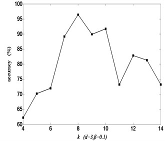
Fig. 4Recognition rate with dimension d
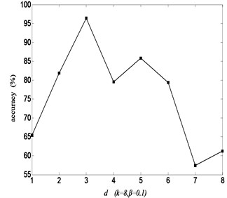
Fig. 5Recognition rate with parameter β
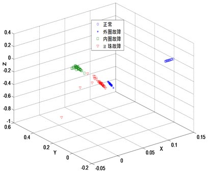
The three-dimensional sensitive features of bearing high-dimensional characteristic samples reduced by LCWR according to the optimized values of 8, 3 and 0.1 are shown in Fig. 6. After dimension reduction, four kinds of bearing samples have no intersection and overlap. Each of them has its own clustering center. The clustering effect and global geometric structure are objective, displaying a distinct manifold structure.
Fig. 6Embedded 3 dimensions by LCWR (k= 8, β= 0.1)
3.3. Dimensionality reduction effect analysis
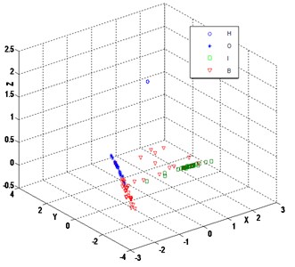
LCWR is compared with LTSA, locally linear embedding (LLE) and principal component analysis (PCA) to verify its dimensionality reduction effect. The dimensionality reduction results of LTSA, LLE and PCA are shown in Fig. 7, Fig. 8, and Fig. 9, respectively. Generally speaking, the reduced dimensionality samples via these methods have different degrees of intersection and overlap, poor clustering within class, lack of clustering centers. It is difficult to mine the essential characteristics of the bearing state and the differences between classes. Although LTSA and LLE find the manifold structure of high-dimensional samples, they are unable to expand the gaps between dissimilar samples in neighborhood. PCA belongs to one of linear statistical distributions without considering the local structure of the samples. It makes the intraclass aggregation poor and the differences between classes unclear, which fails to reveal the non-linear manifold structure of the bearing state as shown in Fig. 9.
Fig. 7Embedded 3 dimensions by LTSA (k= 9)
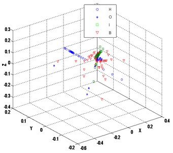
Fig. 8Embedded 3 dimensions by LLE (k= 5)
Combining its weight coefficient with local coordinate’s permutation, LCWR enhances the intraclass aggregation and the differences between classes, overcomes the shortcomings that LTSA and LLE can’t enlarge the gaps between dissimilar samples in neighborhood, simplifies the dimension while retaining the low-dimensional principal characteristics of high-dimensional samples, accurately reflects the relationship between signal characteristics and the bearing state, and effectively distinguishes four kinds of bearing states. As shown in Table 2, the features extracted by various methods are sent to SVM and the recognition rate of LCWR reaches the highest 96.43 % despite a little more time to run LCWR than LTSA, LLE and PCA as shown in Table 3. Therefore, in contrast to other dimensionality reduction methods, LCWR can achieve higher accuracy and prove its effectiveness.
Fig. 9Embedded 3 dimensions by PCA
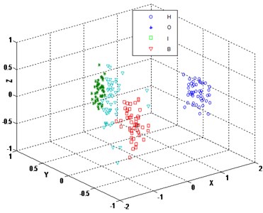
Table 2Bearing condition recognition rate with various methods (%)
Sample | LCWR (8, 3, 0.1) | LTSA (9, 3) | LLE ( 5, 3) | PCA (3) | NDR ( 20) |
H vs. (O+I+B) | 100 | 100 | 100 | 100 | 75 |
O vs. (I+B) | 93.06 | 93.06 | 95.83 | 97.22 | 66.67 |
B vs. (O+I) | 93.06 | 66.67 | 80.56 | 66.67 | 72.22 |
I vs. (O+B) | 97.22 | 95.83 | 87.50 | 94.44 | 95.83 |
I vs. B | 95.83 | 93.75 | 85.42 | 91.67 | 91.67 |
O vs. I | 100 | 95.83 | 93.75 | 100 | 95.83 |
O vs. B | 95.83 | 85.41 | 93.75 | 89.58 | 95.83 |
Average rate | 96.43 | 90.08 | 90.97 | 91.37 | 84.72 |
H-healthy, O-outer race defect, I-inner race defect, B-ball defect, NDR-non dimensionality reduction | |||||
Table 3Running time of SVM combined with various methods (s)
Sample | LCWR (8, 3, 0.1) | LTSA (9, 3) | LLE ( 5, 3) | PCA (3) | NDR ( 20) |
H vs. (O+I+B) | 66 | 27 | 28 | 26 | 57 |
O vs. (I+B) | 73 | 27 | 31 | 26 | 78 |
B vs. (O+I) | 74 | 37 | 31 | 39 | 71 |
I vs. (O+B) | 69 | 26 | 26 | 27 | 58 |
I vs. B | 70 | 26 | 26 | 25 | 59 |
O vs. I | 62 | 24 | 26 | 24 | 56 |
O vs. B | 67 | 27 | 30 | 26 | 70 |
Average time | 71 | 28 | 28 | 28 | 64 |
Besides, it can be founded that recognition rate of manifold dimensionality reduction using LCWR, LTSA, LLE and PCA (all greater than 90 %) is higher than that of the non-dimensionality reduction method (only 84.72 %). It is further proved that these manifold learning methods can filter redundancy and interference of the high-dimensional features and extract the intrinsic low-dimensional manifold characteristics, which can significantly improve the recognition rate of the bearing state as shown in Table 2. Meanwhile, these manifold learning methods except LCWR consume less time and get better recognition efficiency.
4. Conclusions
LCWR manifold learning is proposed to remove redundancy and noise in bearing high-dimensional fault features and perform non-linear dimensionality reduction for improvement in fault diagnosis capability. Geodesic distance based weight function is used to realign local coordinates to eliminate redundancy and interference in high-dimensional feature samples and extract low-dimensional sensitive fault features. Experiments demonstrate that the intrinsic manifold structure of high-dimensional feature samples can be well preserved after dimensionality reduction by LCWR, and the extracted low-dimensional feature samples can truly represent the non-linear characteristics of different bearing states and the gaps between them. The low-dimensional feature samples are then identified by SVM, which results in a higher recognition rate than other methods. Thus, the effectiveness of LCWR is validated. In addition, LCWR is worth further studying to save running time.
References
-
Randall R. B., Antoni J. Rolling element bearing diagnostics – a tutorial. Mechanical Systems and Signal Processing, Vol. 25, Issue 2, 2011, p. 485-520.
-
Dolenc B., Boškoski P., Juričić D. Distributed bearing fault diagnosis based on vibration analysis. Mechanical Systems and Signal Processing, Vols. 66-67, 2016, p. 521-532.
-
Wu C. X., Chen T. F., Jiang R., Ning L. W., Jiang Z. A novel approach to wavelet selection and tree kernel construction for diagnosis of rolling element bearing fault. Journal of Intelligent Manufacturing, Vol. 28, Issue 8, 2017, p. 1847-1858.
-
Kumar R., Singh M. Outer race defect width measurement in taper roller bearing using discrete wavelet transform of vibration signal. Measurement, Vol. 46, Issue 1, 2013, p. 537-545.
-
Kankar P. K., Sharma S. C., Harsha S. P. Rolling element bearing fault diagnosis using autocorrelation and continuous wavelet transform. Journal of Vibration and Control, Vol. 17, Issue 14, 2011, p. 2081-2094.
-
Patel V. N., Tandon N., Pandey R. K. Defect detection in deep groove ball bearing in presence of external vibration using envelope analysis and Duffing oscillator. Measurement, Vol. 45, Issue 5, 2012, p. 960-970.
-
Wang Y., Xu G. H., Liang L., Jiang K. S. Detection of weak transient signals based on wavelet packet transform and manifold learning for rolling element bearing fault diagnosis. Mechanical Systems and Signal Processing, Vol. 54, Issue 55, 2015, p. 259-276.
-
Wang J., He Q. B., Kong F. R. Multiscale envelope manifold for enhanced fault diagnosis of rotating machines. Mechanical Systems and Signal Processing, Vol. 52, Issue 53, 2015, p. 376-392.
-
Jiang Q. S., Jia M. P., Hu J. Z., Xu F. Y. Machinery fault diagnosis using supervised manifold learning. Mechanical Systems and Signal Processing, Vol. 23, Issue 7, 2009, p. 2301-2311.
-
Wang C., Gan M., Zhu C. G. Non-negative EMD manifold for feature extraction in machinery fault diagnosis. Measurement, Vol. 70, 2015, p. 188-202.
-
Zhang Z. Y., Zha H. Y. Principal manifolds and nonlinear dimension reduction via local tangent space alignment. Journal of Shanghai University, Vol. 8, Issue 4, 2004, p. 406-424.
-
Wang Q., Wang W. G., Nian R., He B., Shen Y., Björk K. M., Lendasse A. Manifold learning in local tangent space via extreme learning machine. Neurocomputing, Vol. 174, 2016, p. 18-30.
-
Zhang P., Qiao H., Zhang B. An improved local tangent space alignment method for manifold learning. Pattern Recognition Letters, Vol. 32, Issue 2, 2011, p. 181-189.
-
Zhang Y., Li B. W., Wang W., Sun T., Yang X. Y., Wang L. Supervised locally tangent space alignment for machine fault diagnosis. Journal of Mechanical Science and Technology, Vol. 28, Issue 8, 2014, p. 2971-2977.
-
Li F., Tang B. P., Yang R. S. Rotating machine fault diagnosis using dimension reduction with linear local tangent space alignment. Measurement, Vol. 46, Issue 8, 2013, p. 2525-2539.
-
Kumar A., Kumar R. Manifold learning using linear local tangent space alignment (LLTSA) Algorithm for noise removal in wavelet filtered vibration signal. Journal of Nondestructive Evaluation, Vol. 35, Issue 3, 2016, p. 50.
-
Su Z. Q., Tang B. P., Liu Z. R., Qin Y. Multi-fault diagnosis for rotating machinery based on orthogonal supervised linear local tangent space alignment and least square support vector machine. Neurocomputing, Vol. 157, 2015, p. 208-222.
-
Wang G. B., Zhao X. Q., He Y. H. Fault diagnosis method based on supervised incremental local tangent space alignment and SVM. Applied Mechanics and Materials, Vols. 34-35, 2010, p. 1233-1237.
-
Su Z. Q., Tang B. P., Deng L., Liu Z. R. Fault diagnosis method using supervised extended local tangent space alignment for dimension reduction. Measurement, Vol. 62, 2015, p. 1-14.
About this article
The work was supported by A Project Supported by Scientific Research Fund of Hunan Provincial Education Department (20A107), Project of National Natural Science Foundation of China (51875193) and Xiangtan guiding science and technology plan project (ZDX-CG2019004). The authors thank all reviewers for their valuable comments and constructive advice on this paper.
