Fault diagnosis using an improved fusion feature based on manifold learning for wind turbine transmission system

Ma, Ping; Zhang, Hongli; Fan, Wenhui; Wang, Cong

doi:10.21595/jve.2019.20132

Journal of Vibroengineering

Browse Journal

Submit article

Published: 15 November 2019

Check for updates

Fault diagnosis using an improved fusion feature based on manifold learning for wind turbine transmission system

Ping Ma¹

Hongli Zhang²

Wenhui Fan³

Cong Wang⁴

^{1, 2, 4}College of Electrical Engineering, Xinjiang University, Urumqi, China

³Department of Automation, Tsinghua University, Beijing, China

Corresponding Author:

Ping Ma

Cite the article Download PDF

Downloads 1526

WoS Core Citations 4

CrossRef Citations 5

Abstract

In this paper, a novel fault diagnosis method based on vibration signal analysis is proposed for fault diagnosis of bearings and gears. Firstly, the ensemble empirical mode decomposition (EEMD) is used to decompose the vibration signal into several subsequences, and a multi-entropy (ME) is proposed to make up the fusion features of the vibration signal. Secondly, an improved manifold learning algorithm, local and global preserving embedding (LGPE), is applied to compress the high-dimensional fusion feature set into a two-dimension feature set. Finally, according to the clustering accuracy of different feature set, the fault classification and diagnosis can be performed in the reduced two-dimension space. The performance of the proposed technique is tested on the fault of wind turbine transmission system. The application results indicate that the proposed method can achieve high accuracy of fault diagnosis.

1. Introduction

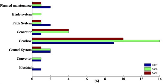
Wind energy as a new clean energy source is the fastest-growing energy source in the world, this trend should endure for some time. However, wind turbines are long-term operated in harsher environments, have relatively higher failure rates. Fig. 1 shows the percentage of downtime with different failure per year at the Dutch wind farm during 3 years operation [1]. It can be seen that the primary causes of failure are damage to the gearbox, generator and faults with the control and pitch systems. The bearings and gears are important parts of those systems, which faults will inevitably cause a long downtimes and increase operating costs. Therefore, proposing a timely and accurate diagnosis method to detect those faults are extremely available, which will reduces energy losses, improves productively and increases safety of such systems [2, 3].

The techniques based on vibration signal analysis are the most popular and useful approaches applied in fault diagnosis of rotating machinery [4-6]. In general, the processing of fault diagnosis can be divided into three steps: data collection, feature extraction and classification. Feature extraction is a key step, which can extract more useful information of the vibration signals from their original measured space for fault diagnosis. Some self-adaptive time-frequency analysis methods have been proposed for fault diagnosis. Empirical mode decomposition (EMD) [7], which were carried out to decompose vibration signals into the sum of intrinsic mode functions (IMF) given different frequencies, and some IMFs containing fault feature frequencies are selected to reconstruct a new signal for outstanding fault feature for further analysis [8, 9]. But the decomposed process of EMD is sensitive to noise and has exist mode mixing problem. Ensemble empirical mode decomposition (EEMD) is a newly improved version of EMD, which can eliminate the mode mixing problem of EMD automatically [10]. This approach has been applied in signal analysis of rotating machinery [11-14]. In conclusion, the self-adaptive time-frequency analysis method EEMD can extract sensitive features and improve the fault diagnosis accuracy.

Fig. 1Downtimes for the Dutch wind farm Egmond aan Zee

The vibration signals collected from wind turbine transmission systems are complex and non-stationary, which are submerged in noise under the variable speeds conditions. Therefore, the fault features from the original signal cannot be comprehensively extracted using single or single-domain processing methods [15, 16]. Therefore, the mix-domain features fusion is proposed to construct high-dimensional feature set. However, the high-dimensional feature set of mixed-domain inevitably contains redundant and disturbed information, and the accuracy of fault diagnosis can be reduced using the high dimensional feature set for pattern recognition. Using an appropriate dimensionality reduction method to extract the main eigenvectors with low dimension, high sensitivity and good clustering characteristics from the high-dimensional feature set for fault recognition is necessary.

Manifold learning [17-20], an effective nonlinear dimension reduction method has gained attention in various research fields. The idea of manifold learning is to project the original high dimensional data into a lower dimension feature space with the local neighborhood structure preserved. This technique including several mainstream algorithms such as locally linear embedding (LLE) [18], locality preserving projection (LPP) and kernel locality preserving projection (KLPP) [20]. Manifold learning is widely used in the filed of image recognition and data classification [21, 22], and there are few researches in fault diagnosis [23, 24]. Due to the advantages of the time-frequency analysis and manifold learning techniques in dealing with non-linear signal, some research works combined fault diagnosis models with time-frequency analysis techniques and dimensionality reduction techniques. Su et al. [25] combined EMD, incremental enhanced supervised locally linear embedding and adaptive nearest neighbor classifier to build a new method for gearbox fault diagnosis. Ding et al. [26] presented a fusion feature extraction method on rolling bearings based on wavelet packet transform and LPP. The classification result shows that this method can enhance the discrimination between all fault classes for fault classification. Huang et al. [27] used a new technique for dimensionality reduction called the discriminate diffusion maps analysis, compared with other manifold learning algorithms, which has high classification accuracy of the bearings faults.

In the above literatures, at the process of feature extraction, the dimensionality reduction methods of manifold learning, which embed the original high-dimensional data into a lower dimension feature space with considering the local nonlinear characteristics preserved. But undeniably, in the process of reducing dimensionality, in order to extract more abundant information, it is necessary to preserve the intrinsic structure and extract the structure of the high-dimensional set.

In this paper, a novel fault diagnosis model based on fusion feature and manifold learning is proposed. Firstly, EEMD is used to decompose the vibration signals into a set of intrinsic mode functions (IMFs) with different characteristics scales, and several IMFs that containing more sensitive information are selected. Secondly, envelope entropy, permutation entropy and energy entropy of those selected IMFs are extracted as representative fusion features. Thirdly, local and global preserving embedding (LGPE), is applied to extract the main eigenvectors from the high-dimensional fusion feature set. This method considers the local nonlinear characteristics and global external structure of the fusion feature set. The feature space dimension is optimally reduce to a low dimensional space by using LGPE, achieving the classification and identification of the fault. The proposed method is verified on the fault diagnosis of the bearing’s and gearbox’s signals.

The main contributions of the proposed method are presented as follows:

1) A fusion feature set is established based on EEMD and Mutli-entropy, in which the fault features can be comprehensively extracted from mixed time-domain signals.

2) A LGPE method is proposed to extract fault features from the high-dimensional feature set, which makes the fault features in low dimensional space has high sensitivity and good clustering characteristics.

3) A novel fault diagnosis model based on EEMD-ME and LGPE is performed to diagnose the faults of bearings and gears, which accurately achieves the identification and classification of different faults.

The organization of the rest of the paper is as follows. In Section 2, the EEMD, ME and LGPE are presented. Section 3 describes the proposed model for fault diagnosis. In Section 4, two fault diagnosis experiments are carried out to verify our proposed method, and the experimental result is discussed. The conclusions are appeared in Section 5.

2. The proposed fault diagnosis model

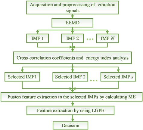
Fig. 2 shows the flow chart of the proposed fault diagnosis method. The relative methods including EEMD, ME and LGPE are presented in this section.

Fig. 2The fault diagnosis process of the proposed method

2.1. Ensemble empirical mode decomposition (EEMD)

EEMD is a non-linear multi-resolution self-adaptive decomposition technique, which can adaptively decompose a complex signal into a set of IMF. The vibration signal of the rotating machinery is nonlinear, non-stationary and submerged in heavy noise, which makes it difficult to detect faults using the original signal. Therefore, EEMD is proposed to decompose the vibration signal into several IMFs with different frequencies for further analysis.

The principle of the EEMD is simple: in the process of decomposition, the frequency scales are natural separated by adding white noise in the whole time-frequency space uniformly, which can reduce the occurrence of mode mixing. The decomposition steps of EEMD is as follows:

Step 1: Add a white noise series $n_{i} (t)$ with zero mean and equal variance to the original vibration signal $x (t)$ :

1

x_{i} (t) = x (t) + n_{i} (t),

where $n_{i} (t)$ represents the $i$ th added white noise series, and $x_{i} (t)$ denotes the noise-added signal of the $i$ th trial, while $i =$ 1, 2, …, $M$ , $M$ is the number of ensemble.

Step 2: Each noise-added signal $x_{i} (t)$ is decomposes into several IMFs using EMD:

2

x_{i} (t) = \sum_{s = 1}^{S} c_{i s} (t) + r_{i S} (t),

where $S$ represents the number of IMF, $s =$ 1, 2, …, $S$ . $c_{i s} (t)$ denotes the IMFs $(c_{i 1}, c_{i 2}, \dots, c_{i S})$ with different frequency bands, and $r_{i S} (t)$ is the residue of $x_{i} (t)$ .

Step 3: Repeat step 1 and step 2 with M times, the different white noise series is added to the signal $x (t)$ to obtain an ensemble of IMFs $[{c_{1 s} (t), c_{2 s} (t), \dots, c_{M s} (t)}]$ .

Step 4: Obtain the ensemble means of the corresponding IMFs as the final IMFs:

3

c_{s} (t) = \frac{1}{M} \sum_{i = 1}^{M} c_{i s} (t),

where $c_{s} (t)$ represents the $i$ th IMF decomposed by EEMD, while $s =$ 1, 2, …, $S$ .

In order select the IMF that containing useful feature information for further analysis, the cross-correlation coefficient $ρ$ and energy index $E$ are introduced to eliminate illusive IMF. Cross-correlation coefficient $a$ is common used in signals analysis and is no longer discussed in here. For a IMF obtained by EEMD, the energy index $E (s)$ is defined as follows:

4

E (s) = \sqrt{\frac{\sum_{t = 1}^{N} {|c_{s} (t)|}^{2}}{\sum_{t = 1}^{N} {|x (t)|}^{2}}},

where $N$ is the length of the signal, $c_{s} (t)$ denotes the $s$ th IMF, and $E (s)$ represents the index of energy between the $s$ th IMF $c_{s} (t)$ and the original signal $x (t)$ .

2.2. Mutil-entropy

The entropy-based methods, such as envelope entropy, energy entropy and permutation entropy [28-30], have been applied in fault diagnosis. In this section, envelope entropy, energy entropy and permutation entropy of the selected IMFs obtained from section 2.1 are extracted as the fusion features of fault signal.

Entropy can identify nonlinear parameters and present the information of the signal, and envelope entropy can reflect the sparseness of the original signal. The envelope entropy $H_{1} (s)$ of a IMF $c_{s} (t) (t = 1,2, \dots, N)$ can be expressed as:

5

\{\begin{array}{l} H_{1} (s) = - \sum_{t = 1}^{N} p_{t} l g p_{t}, \\ p_{t} = \frac{a (t)}{\sum_{t = 1}^{N} a (t),} \end{array}

where $a (t)$ is the envelope signal that obtained by the Hilbert demodulation of signal $c_{s} (t)$ , $p_{t}$ is the normalized form of signal $c_{s} (t)$ .

In the same way, the energy entropy of the IMF $c_{s} (t)$ , which can be defined as:

6

H_{2} (s) = - \sum_{s = 1}^{S} p_{s} l o g p_{s},

where $p_{s} = E (s) / E$ is the proportion of the energy of the $s$ th IMF in the whole signal energies.

Permutation entropy (PE) is used to analyze the data complexity. For a IMF $c_{s} (t)$ , constructing an embedded d-dimensional delay embedding matrix $C_{d} (t) = \{x_{t + σ}, x_{t + 2 σ}, \cdot \cdot \cdot, x_{t + d σ}\}$ , and arranging each vector of $C_{d}$ to an increasing order $C_{i} (t) = \{c_{i + j_{1}} \leq c_{i + j_{2}} \leq \cdot \cdot \cdot \leq c_{i + j_{d}}\}$ . Letting $π_{i} = (j_{1}, j_{2}, \dots, j_{d})$ , which is one of the $d$ ! permutations of $d$ distinct symbols. Then the permutation entropy of IMF $c_{s} (t)$ , with the probability distribution function $p (π_{i})$ is defined as:

7

H_{3} (s) = - \sum_{i}^{n - σ d + 1} p (π_{i}) \ln (p (π_{i})) .

2.3. Local and global preserving embedding (LGPE) algorithm

The generic reduction problem of feature space dimension is described as follows: let a $n$ -dimension points $X = [x_{1}, x_{2}, \dots, x_{n}] \in R^{n}$ , which can be transformed into an $d$ -dimension $Y = [y_{1}, y_{2}, \dots, y_{d}] \in R^{d}$ , $(d < n)$ , where $y_{i} = W^{T} x_{i}$ , and $W$ is an transformation matrix. In this section, a novel dimensionality reduction method, LGPE is used to project a manifold in high-dimensional space $R^{n}$ to a low-dimensional space $R^{d}$ while preserving the local neighborhood and global structure of the dataset.

The objective function of the LGPE can be divided into two parts: the local nonlinear characteristics preservation objective function and the global variance maximum objective function. The local nonlinear characteristics preservation objective function makes the low-dimension feature space has the similar neighborhood structure with high-dimensional feature space. The global variance maximum objective function extracts the maximize variance of the data during the dimensionality reduction process.

2.3.1. The local nonlinear characteristics preservation objective function

Given a set of data $X = [x_{1}, x_{2}, \dots, x_{n}] \in R^{n}$ , $x_{i}$ is a $n$ -dimensional feature vector. Firstly, we use a possibly nonlinear function $ϕ$ to map the data into a high-dimension feature space $H$ : $ϕ (X) = [ϕ (x_{1}), ϕ (x_{2}), \dots, ϕ (x_{n})]$ . Inspired by the idea of kernel locality preserving projection (KLPP), we seek a projecting transformation $W$ , which can preserve the local nonlinear structure of the data $ϕ (x)$ by minimizing the sum of the weighted distance of samples. The minimization problem of local nonlinear characteristics preservation objective function can be expressed as:

8

J_{l o c a l} (W) = \underset{W}{m i n} \sum_{i, j = 1}^{N} {‖y_{i} - y_{j}‖}^{2} S_{i, j},

where $y_{i} = (ϕ (x))^{T} W$ is the low-dimension projection of $ϕ (x)$ onto $W$ . $S$ represents a weight matrix, which is constructed through the nearest-neighbor graph. It is defined as follows:

9

S_{i, j} = \{\begin{array}{l} \frac{e x p (- {‖ϕ (x_{i}) - ϕ (x_{j})‖}^{2})}{t} ϕ (x_{i}), ϕ (x_{j}) as neighbors, \\ 0, other, \end{array}

where $t$ is a suitable constant. $S_{i, j}$ denotes the relationship of $ϕ (x_{i})$ and $ϕ (x_{j})$ . The objective Eq. (7) can be transformed as:

10

\begin{array}{l} J_{l o c a l} (W) = \underset{W}{m i n} \sum_{i, j = 1}^{N} {‖y_{i} - y_{j}‖}^{2} S_{i, j} = \underset{W}{m i n} \sum_{i, j = 1}^{N} {‖(ϕ (x_{i}))^{T} W - (ϕ (x_{j}))^{T} W‖}^{2} S_{i, j} \\ = \underset{W}{m i n} {W^{T} (ϕ (X))^{T} (D - S) (ϕ (X)) W\}, \end{array}

where $D_{i i} = \sum_{j} S_{i, j}$ is a diagonal matrix. Because the projecting transformation $W$ must be in the span of $ϕ (x_{1}), ϕ (x_{2}), \dots, ϕ (x_{n})$ , there have a coefficient vector $A = (a_{1}, a_{2}, \dots, a_{n})^{T}$ to satisfy the equation $W = \sum_{j = 1}^{n} a_{j} ϕ (x_{j}) = ϕ (X)^{T} A$ . Then the local nonlinear characteristics preservation objective function can be expressed as:

11

\begin{array}{l} J_{l o c a l} (A) = \underset{A}{m i n} {A^{T} ϕ (X) (ϕ (X))^{T} (D - S) ϕ (X) (ϕ (X))^{T} A} \\ = \underset{A}{m i n} {A^{T} ϕ (X) (ϕ (X))^{T} L ϕ (X) (ϕ (X))^{T} A\}, \end{array}

where $L = D - S$ is a Laplacian matrix. In order to solve this nonlinear problem, a positive definite and symmetric kernel matrix $K (i, j) = ϕ (x_{i}) \cdot ϕ (x_{j})^{T}$ is introduced to the Eq. (11). The objective Eq. (11) can be calculated as:

12

J_{l o c a l} (A) = \underset{A}{m i n} A K L K A = \underset{α}{m i n} A^{T} L_{l} A, (L_{1} = K L K) .

The local nonlinear structure of the high-dimension dataset is preserved by keeping the nearest neighbor relation of the dataset in the kernel space. It is obvious that, the solution of local nonlinear characteristics preservation objective function will keep the local structural characteristics of dataset in the process of dimensionality reduction.

2.3.2. The global variance maximum objective function

Given a set of data $X = [x_{1}, x_{2}, \dots, x_{n}] \in R^{n}$ , and using a possibly nonlinear function $ϕ$ to map the data into a high-dimension feature space $H$ : $ϕ (X) = [ϕ (x_{1}), ϕ (x_{2}), \dots, ϕ (x_{n})]$ . Inspired by the idea of kernel principal component analysis (KPCA), the global variance maximum objective function $J_{g l o b a l} (W)$ is defined as: seeking a projecting transformation $W$ , which makes the matrix $y_{i} = (ϕ (x_{i}))^{T} W$ after projection preserves the maximum variance information for the high-dimension data $ϕ (x)$ . Then the optimization task can be expressed as:

13

\begin{array}{l} J_{g l o b a l} (W) = \underset{W}{m a x} \sum_{i = 1}^{n} y_{i}^{2} = \underset{W}{m a x} \sum_{i = 1}^{n} ((ϕ (x_{i}))^{T} W)^{2}, \\ s . t . W^{T} W = 1 . \end{array}

It is well known that exist a coefficient vector $A = (a_{1}, a_{2}, \dots, a_{n})^{T}$ to satisfy the equation $W = \sum_{j = 1}^{n} a_{j} ϕ (x_{j}) = ϕ (X)^{T} A$ . Substituting this equation into Eq. (13), the optimization problem transformed into:

14

\begin{array}{l} J_{g l o b a l} (A) = \underset{W}{m a x} \sum_{i = 1}^{n} {((ϕ (x_{i}))^{T} \sum_{j = 1}^{n} a_{j} ϕ (x_{j}))}^{2}, \\ s . t . {(\sum_{j = 1}^{n} a_{j} ϕ (x_{j}))}^{T} (\sum_{j = 1}^{n} a_{j} ϕ (x_{j})) = 1, \end{array}

with the introduction of the kernel function $K (i, j) = ϕ (x_{i}) \cdot ϕ (x_{j})^{T}$ , the Eq. (14) can be expressed as:

15

\begin{array}{l} J_{g l o b a l} (A) = \underset{W}{m a x} \sum_{i = 1}^{n} {(\sum_{j = 1}^{n} a_{j} K (i, j))}^{2}, \\ s . t . \sum_{i = 1}^{n} \sum_{j = 1}^{n} a_{i} a_{j} K (i, j) = 1, \end{array}

we can further express Eq. (15) as:

16

\begin{array}{l} J_{g l o b a l} (A) = \underset{W}{m a x} A^{T} K K A = \underset{W}{m a x} A^{T} C A, \\ s . t . A^{T} K A = 1 . \end{array}

2.3.3. The objective function of LGPE

In order to preserve the local nonlinear structure between neighboring data points and extract the variance of the maximal high-dimension data, the objective function of the LGPE is to minimize $A^{T} L_{l} A$ (for local structure preserving) and maximize $A^{T} K K A$ (for global variance extracting). The objective function of LGPE can be transformed to the following optimization problem:

17

\begin{array}{l} J (A) = \underset{A}{m a x} (J_{g l o b a l} (A) - J_{l o c a l} (A)) = \underset{A}{m a x} (A^{T} C A - A^{T} L_{1} A) = \underset{A}{m a x} (A^{T} (C - L_{1}) A), \\ s . t . A^{T} K A = 1 . \end{array}

In order to eliminate the influence of noise in the process of dimensionality reduction, an orthogonal constraint is introduced. The derivation process is inspired by literature [31]:

18

α_{1}^{T} α_{k} = α_{2}^{T} α_{k} = \cdot \cdot \cdot = α_{k - 1}^{T} α_{k} = 0 .

In order to obtain the $k$ orthogonal basis vector $α_{k}$ , the following objective function need to be minimized:

19

\begin{array}{l} \underset{α}{J (α) = m a x} ({α_{n}}^{T} (C - L_{1}) α_{n}), \\ s . t . α_{1}^{T} α_{k} = α_{2}^{T} α_{k} = \cdot \cdot \cdot = α_{k - 1}^{T} α_{k} = 0, \\ α_{1}^{T} K α_{1} = α_{2}^{T} K α_{2} = \cdot \cdot \cdot = α_{k}^{T} K α_{k} = 1 . \end{array}

In order to compute the $n$ th discriminant vector, the lagrange multipliers in introduced to transform the $J_{α}$ . criterion including all the constraints:

20

J_{α} = α_{k}^{T} (C - L_{1}) α_{k} - λ (α_{k}^{T} K α_{k} - 1) - \sum_{i = 1}^{k - 1} μ_{i} α_{k}^{T} α_{i} .

The optimization is performed by setting the partial derivative of $J_{α}$ with respect to $α_{k}$ equal to zero:

21

\frac{\partial L_{k}}{\partial α_{k}} = 0 \Rightarrow 2 (C - L_{1}) α_{k} - 2 λ K α_{k} - \sum_{i = 1}^{k - 1} μ_{i} α_{i} = 0 .

Multiplying the left side of Eq. (21) by $α_{k}^{T}$ obtained:

22

2 α_{k}^{T} (C - L_{1}) α_{k} - 2 λ α_{k}^{T} K α_{k} = 0 \Rightarrow λ = \frac{α_{k}^{T} (C - L_{1}) α_{k}}{α_{k}^{T} K α_{k}} .

Multiplying the left side of Eq. (21) successively by $α_{1}^{T} K^{- 1}$ , $α_{2}^{T} K^{- 1}$ , …, $α_{k - 1}^{T} K^{- 1}$ , and obtaining a set of $k - 1$ expressions:

23

\begin{array}{l} μ_{1} α_{1}^{T} K^{- 1} α_{1} + \cdot \cdot \cdot + μ_{k - 1} α_{1}^{T} K^{- 1} α_{k - 1} = 2 α_{1}^{T} K^{- 1} (C - L_{1}) α_{k}, \\ μ_{1} α_{2}^{T} K^{- 1} α_{1} + \cdot \cdot \cdot + μ_{k - 1} α_{2}^{T} K^{- 1} α_{k - 1} = 2 α_{2}^{T} K^{- 1} (C - L_{1}) α_{k}, \\ ⋮ \\ μ_{1} α_{k - 1}^{T} K^{- 1} α_{1} + \cdot \cdot \cdot + μ_{k - 1} α_{1}^{T} K^{- 1} α_{k - 1} = 2 α_{k - 1}^{T} K^{- 1} (C - L_{1}) α_{k} . \end{array}

Define the matrix notation:

U_{k - 1} = [μ_{1}, μ_{2}, \dots, μ_{k - 1}]^{T}, α = (α_{1}, α_{2}, \dots, α_{k - 1})^{T}, M_{k - 1} = [M_{i j}^{k - 1}], M_{i j}^{k - 1} = α_{i}^{T} K^{- 1} α_{j} .

Then the equations can be transformed in a single matrix relationship:

24

M_{k - 1} U_{k - 1} = 2 α_{k - 1}^{T} K^{- 1} (C - L_{1}) α_{k} .

Or in another form:

25

U_{k - 1} = 2 (M_{k - 1})^{- 1} α_{k - 1}^{T} K^{- 1} (C - L_{1}) α_{k} .

Multiply the left side of Eq. (21) by $K^{- 1}$ :

26

2 K^{- 1} (C - L_{1}) α_{k} - 2 λ α_{k} - K^{- 1} α_{k - 1} U_{k - 1} = 0 .

Including Eq. (26), we can obtained:

27

K^{- 1} (C - L_{1}) α_{k} - K^{- 1} α_{k - 1} (M_{k - 1})^{- 1} α_{k - 1}^{T} K^{- 1} (C - L_{1}) α_{k} = λ α_{k} .

Or in another form:

28

(I - K^{- 1} α_{k - 1} M_{k - 1}^{- 1} α_{k - 1}^{T}) K^{- 1} (C - L_{1}) α_{k} = λ α_{k} .

We need to maximized the criterion $λ$ of Eq. (28):

29

R_{k} = (I - K^{- 1} α_{k - 1} M_{k - 1}^{- 1} α_{k - 1}^{T}) K^{- 1} (C - L_{1}) .

Thus, the required the $k$ orthogonal basis vector $α_{k}$ is the eigenvector corresponding to the maximum eigenvalue of $R_{k}$ . It is easy to verify that $α_{1}$ is the eigenvector corresponding to the minimum eigenvalue of the generalized eigenvalue equation $(C - L_{1}) = λ K$ .

3. Fault diagnosis process

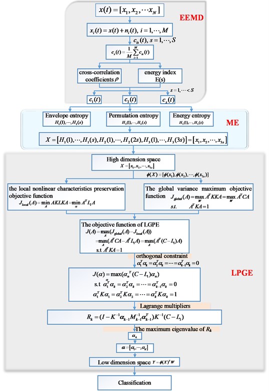
In this study, a novel fault diagnosis model based on EEMD-ME and LGPE is proposed. The detail frameworks are shown in Fig. 3, the procedures of this model is described in successive steps:

Step 1: For a test signal $x_{i} = [x_{1}, x_{2}, \dots, x_{N}]$ , EEMD is used to decompose the signal into several IMFs. Then calculate cross-correlation coefficient and energy index of each IMF, and select the first $s$ IMFs to further analysis.

Step 2: The envelope entropy, permutation entropy and energy entropy of each selected IMFs are combined into an 3s-dimension fusion features $x_{i} = [x_{i 1}, x_{i 2}, \dots, x_{i 3 s}]^{T}$ .

Step 3: The 3s-dimension fusion feature set of test samples is input into LPGE to reduce the high-dimension feature space to two-dimension feature set $Y = [y_{1}, y_{2}]$ . The dimensionality reduction steps are shown as follows:

1) For a high-dimension feature dataset $X = [x_{1}, x_{2}, \dots, x_{3 s}] \in R^{3 s}$ , we can construct the local nonlinear characteristics preservation objective function $J_{l o c a l} (A)$ by using Eq. (12).

2) The global variance maximum objective function $J_{g l o b a l} (A)$ can be obtained by Eq. (16)

3) The objective function of proposed LGPE is defined at Eq. (19), and calculate the $k$ orthogonal basis vector $α_{k}$ of projection matrix $α = (α_{1}, α_{k}, \dots, α_{d})$ by iteration $α_{k}$ is the eigenvector corresponding to the maximum eigenvalue of Eq. (29).

4) According to the equation $y_{i} = (ϕ (x_{i}))^{T} W$ , the low-dimension feature set $Y = [y_{1}, y_{2}]$ after projection space transformation can be obtained.

Step 5: Classify and recognize the different faults by the degree of clustering in two-dimensional space.

Fig. 3The details framework of the proposed model

4. Result and discussion

To investigate the effectiveness of the proposed technology for fault diagnosis, two experimental cases are considered. They including the bearing data obtained from the Case Western Reserve University (CWRU) Bearing Data Center and the gear data produced by QPZZ-II system.

4.1. The fault diagnosis of bearings

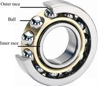
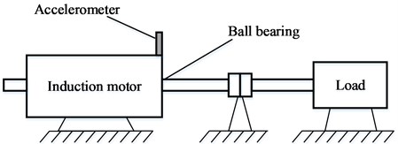
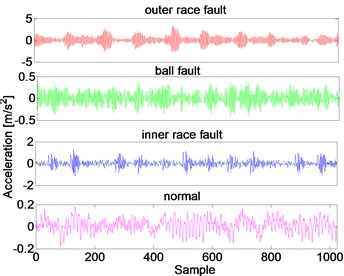
The bearing data obtained from CWRU Bearing Data Center has become a standard preference at the filed of fault diagnosis in bearings. A ball bearing as shown in Fig. 4, which was installed in a motor driven mechanical system. Vibration data is collected using accelerometers, which are attached to the housing with magnetic bases. In total four sets of data are obtained form the experiment systems, which include under normal conditions, with inner race fault, with ball fault and with outer race fault. The sampling frequency is 12 kHz for drive end bearing experiments. In this paper, the 0.007 inches fault diameter is selected for fault diagnosis. The vibration signal obtained from four different conditions are divided into 100 segments of 1024 sample each, as shown in Fig. 5.

Fig. 4Experimental system

a)

b)

Fig. 5Segments of the vibration signals collected from four different conditions of bearing

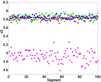
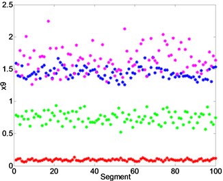
Each segment of vibration signal is decomposed into 10 IMFs by EEMD. For a segment, the cross-correlation coefficients $ρ$ and energy index $E$ of the former 4 IMF are presented in Table 1. It can be noticed that the first 4 IMFs have higher cross-correlation coefficients and energy index, which are chosen as the sensitive components for further analysis. The envelope entropy, permutation entropy and energy entropy of the first 4 IMFs in each segment are extracted as fusion features. In total 12 features are extracted for each segments as a point $x_{i} = (x_{i 1}, x_{i 2}, \dots, x_{i 12})$ in the feature space with the dimension of 12. And these points make up a fusion feature set $X = [x_{1}, x_{2}, \dots, x_{100}]$ in a high-dimension space. Fig. 6(a), (b) and (c) show the envelope entropy, permutation entropy and energy entropy of the IMF1, respectively. In Fig. 6, we can see that the extracted feature have a certain potential for the fault detection at some extent but it also not for a fault diagnosis.

Since none of the extracted feature of 12 respective features is completely suitable for fault diagnosis, it is necessary to extract the features that can achieve a better classification ability between different classes of bearing condition. The idea of LGPE is to find a feature space whose dimension can be reduced without any loss information, and makes the classification process become simple. In this paper, we use the LGPE to solve the classification problem.

Table 1Cross-correlation coefficients and energy index of each IMF

IMFs	Outer race fault		Ball fault		Inner race fault		Normal
–	$ρ$	$E$	$ρ$	$E$	$ρ$	$E$	$ρ$	$E$
1	0.8224	0.8094	0.7125	0.6538	0.7209	0.5833	0.6161	0.4591
2	0.4980	0.4287	0.5783	0.4735	0.7549	0.5519	0.6359	0.4370
3	0.3009	0.2190	0.4225	0.2260	0.4213	0.3071	0.2940	0.1719
4	0.1983	0.1502	0.3084	0.2440	0.1838	0.1126	0.4515	0.3830

Fig. 6a) Envelope entropy, b) permutation entropy, c) energy entropy of the IMF1, outer race fault (red), ball fault (green), inner race fault (blue) and normal (magenta)

a) Envelope entropy, b) permutation entropy, c) energy entropy of the IMF1, outer race fault (red), ball fault (green), inner race fault (blue) and normal (magenta)

a)

b)

c)

In this experiment, the reduce dimensionality of LPGE is set to $d =$ 2, and the number of neighborhood points $k$ is 10. using the mixed-domain feature fusion method EEMD-ME and dimensionality reduction method LPGE, the distribution of the low-dimensional feature set after dimension reduction as shown in Fig. 7(a). As is can be seen in Fig. 7(a), all these four types of samples separated from each other in $d$ -dimension space. The low dimensional feature set of the three fault sample cluster well, which are far away from the normal state. Thus, the fault diagnosis is performed.

The dimension reduction effect of LPGE is compared with other three mainstream dimension reduction algorithms KLPP, KPCA and LPP. The dimensionality reduction parameters of these algorithms are also set to $d =$ 2, $k =$ 10. The distributions of the low-dimensional feature sets after dimension reduction of KLPP, KPCA, LPP are shown in Fig. 7(b)-(d). Both Fig. 7(b), (c) and (d) indicate that KLPP, KPCA and LPP cannot separate the four different type of bearing effectively. As it can be notice that while using KLPP and KPCA, there are some overlaps between the outer race fault and ball fault, and outer race fault is large mixed with the inner race fault while using KPCA. The result proves that LPGE has more excellent clustering and classifying performance than KLPP, KPCA and LPP.

Fig. 7The distribution of the low-dimensional feature sets of bearing after dimensionality reduction of LPGE, KLPP, KPCA and LPP

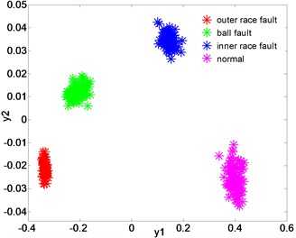
a) Dimensionality reduction with LPGE

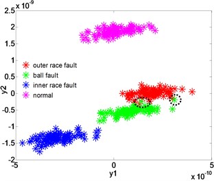
b) Dimensionality reduction with KLPP

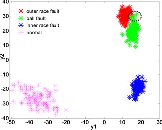
c) Dimensionality reduction with KPCA

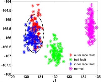
b) Dimensionality reduction with LPP

4.2. The fault diagnosis of gear

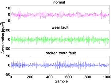
In this experiment, the QPZZ-II test rig is designed to perform the fault test of gears. In total three types of data are obtained from the experiment systems, which include under normal conditions, with wear fault and with broken tooth fault. The sampling frequency is 5120 Hz. Each vibration signal is divided into 50 segments of 1024 sample, as shown in Fig. 8.

Fig. 8Vibration signals collected from three different conditions of the gear

In the same way, each vibration segment of gear signal is decomposed into 10 IMFs by EEMD. Taking one segment as an example, the cross-correlation coefficients $ρ$ and energy index $E$ of each IMF of a segment are presented in Table 2. From it we can see that the first 3 IMFs have higher cross-correlation coefficients and energy index of the original vibrant signal. We select these 3 IMFs as the sensitive components for further analysis. Calculating the envelope entropy, permutation entropy and energy entropy of the first 3 IMFs in each segment. In total 9 features are extracted for each segments as a point $x_{i} = (x_{i 1}, x_{i 2}, \dots, x_{i 9})$ in the feature space with the dimension of 9. And these points make up a feature dataset $X = [x_{1}, x_{2}, \dots, x_{100}]$ in a high-dimension space.

Table 2Cross-correlation coefficients and energy index of each IMF

IMFs	Outer race fault		Ball fault		Inner race fault
–	$ρ$	$E$	$ρ$	$E$	$ρ$	$E$
1	0.6123	0.5342	0.8597	0.8428	0.8915	0.8721
2	0.7907	0.6791	0.5518	0.4315	0.4841	0.3615
3	0.3425	0.2322	0.1907	0.1713	0.2242	0.1835

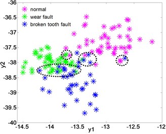
For the gear vibration signal, using EEMD-ME and LPGE, the distribution of the low-dimensional feature set is shown in Fig. 9(a). The proposed method can separate three different gear conditions from each other. At the low dimensional space, the normal sample and the wear fault sample cluster well, while the broken tooth fault sample which are also has a certain degree of dispersion. In general, these samples after dimensionality reduction can effectively achieve the different conditions classification of gears.

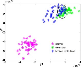
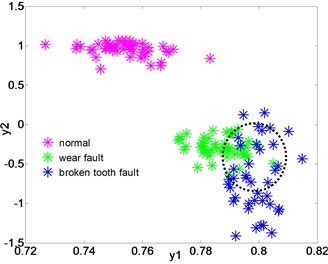
Fig. 9The distribution of the low-dimensional feature sets of gear after dimensionality reduction of LPGE, KLPP, KPCA and LPP

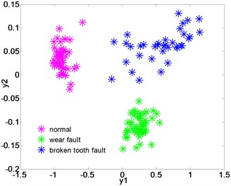
a) Dimensionality reduction with LPGE

b) Dimensionality reduction with KLPP

c) Dimensionality reduction with KPCA

b) Dimensionality reduction with LPP

Fig. 9(b)-(d) show the distribution of the low-dimensional feature set after the dimension reduction of KLPP, KPCA, LPP. In Fig. 9(b)-(d), it can be noticed that both the three methods cannot effectively separate the wear fault and broken tooth fault. In Fig. 9(b) and (c), when using KLPP and KPCA, there are some overlaps between the wear fault and broken fault, and the clustering of the samples with same fault is not well. In Fig. 9(d), the three type samples of gear are mixed together. The result verifies that the LPGE can achieve higher classification accuracy than other methods.

The above results demonstrate the superior performance of the proposed method. Dimensionality reduction with LPGE is better than other classical dimension reduction algorithms. For an online vibration monitoring system, it is necessary to install an automated technique for fault diagnosis. The proposed fault diagnosis model can be used as the core diagnosis strategy of online vibration monitoring systems. Such the system enables an objective, reliable detection and diagnosis of mechanical faults. It also saves time of maintenance technicians and improves the economic performance of the equipment.

5. Conclusions

Bearings and gears are extensively used in wind turbine transmission systems. Defective bearings and gears cause high amplitude of vibration, which can increase power consumption and reduce the economic benefits of rotating machinery. Therefore, a reliable and faster fault diagnosis technique for bearings and gears is important for wind turbine maintenance decisions and reduce operating costs. In this paper, we proposed such a technique to be used for the key components of wind turbine transmission systems. The new technique based on the mixed-domain feature fusion (EEMD-ME) and dimensionality reduction (LPGE) demonstrates a high classification accuracy. The accuracy of the technique was tested on bearing and gear vibration signals. The four classes of the recorded bearing vibration signals, i.e. normal, outer race fault, inner race fault and ball fault operation, and three classes of the recorded gear vibration signals, i.e. normal, wear fault and broken tooth fault operation. The result demonstrates the technology achieves 100 % accuracy.

As part of further work, we plan to introduced the technique into the fault diagnosis of a wind turbine transmission system under variable speeds and alternating loads for wind turbine maintenance decision-making.

References

Wind Energy Report Germany. 2012, https://www.iwes.fraunhofer.de/.

Search CrossRef
Zhao H., Yao R., Xu L., et al. Study on a novel fault damage degree identification method using high-order differential mathematical morphology gradient spectrum entropy. Entropy, Vol. 20, Issue 9, 2018, p. 682.

Publisher
Avendaño Valencia L.-D., Fassois S. D. Damage/fault diagnosis in an operating wind turbine under uncertainty via a vibration response Gaussian mixture random coefficient model based framework, Mechanical System and Signal Processing, Vol. 91, 2017, p. 326-353.

Publisher
Deng W., Yao R., Zhao H., et al. A novel intelligent diagnosis method using optimal LS-SVM with improved PSO algorithm. Soft Computing, 2017, https://doi.org/10.1007/s00500-017-2940-9.

Publisher
Hu A. J., Yan X. A., Xiang L. A new wind turbine fault diagnosis method based on ensemble intrinsic time-scale decomposition and WPT-fractal dimension. Renewable Energy, Vol. 83, 2015, p. 767-778.

Publisher
Deng W., Zhang S., Zhao H., et al. A novel fault diagnosis method based on integrating empirical wavelet transform and fuzzy entropy for motor bearing. IEEE Access, Vol. 6, 2018, p. 35042-35056.

Publisher
Huang N. E., Shen Z., Long S. R., et al. The empirical mode decomposition and the Hilbert spectrum for nonlinear and non-stationary time series analysis. Proceedings of the Royal Society of London A: Mathematical, Physical and Engineering Sciences, Vol. 454, Issue 1971, 1998, p. 903-995.

Publisher
Bin G. F., Gao J. J., Li X. J., Dhillon B. S. Early fault diagnosis of rotating machinery based on wavelet packets – empirical mode decomposition feature extraction and neural network. Mechanical System and Signal Processing, Vol. 27, 2012, p. 696-711.

Publisher
Ricci R., Pennacchi P. Diagnostics of gear faults based on EMD and automatic selection of intrinsic mode functions. Mechanical System and Signal Processing, Vol. 25, Issue 3, 2011, p. 821-838.

Publisher
Wu Z., Huang N. E. Ensemble empirical mode decomposition: a noise-assisted data analysis method. Advances in Adaptive Data Analysis, Vol. 1, Issue 1, 2009, p. 1-41.

Publisher
Lei Y. G., Li Lin et al. N. P. J. Fault diagnosis of rotating machinery based on an adaptive ensemble empirical mode decomposition. Sensor, Vol. 13, 2013, p. 16950-16964.

Publisher
Zhao H., Sun M., Deng W., et al. A new feature extraction method based on EEMD and multi-scale fuzzy entropy for motor bearing. Entropy, Vol. 19, Issue 1, 2016, p. 14.

Publisher
Wang J., Gao R. X., Yan R. Integration of EEMD and ICA for wind turbine gearbox diagnosis. Wind Energy, Vol. 17, Issue 5, 2014, p. 757-773.

Publisher
Imaouchen Y., Kedadouche M., Alkama R., et al. A frequency-weighted energy operator and complementary ensemble empirical mode decomposition for bearing fault detection. Mechanical System and Signal Processing, Vol. 82, 2017, p. 103-116.

Publisher
Chen J. L., Pan J., Li Z. P., Zi Y. Y., Chen C. F. Generator bearing fault diagnosis for wind turbine via empirical wavelet transform using measured vibration signals. Renewable Energy, Vol. 89, 2016, p. 80-92.

Publisher
Tang B. P., Song T., Li F., Deng L. Fault diagnosis for a wind turbine transmission system based on manifold learning and Shannon wavelet support vector machine. Renewable Energy, Vol. 62, 2014, p. 1-9.

Publisher
Tenenbaum J. B., De Silva V., Langford J. C. A global geometric framework for nonlinear dimensionality reduction. Science, Vol. 290, Issue 5500, 2000, p. 2319-2323.

Publisher
Roweis S. T., Saul L. K. Nonlinear dimensionality reduction by locally linear embedding. Science, Vol. 290, Issue 5500, 2000, p. 2323-2326.

Publisher
Seung H. S., Lee D. D. The manifold ways of perception. Science, Vol. 290, Issue 5500, 2000, p. 2268-2269.

Publisher
He X., Niyogi P. Locality preserving projections. Advances in Neural Information Processing Systems, 2004, p. 153-160.

Search CrossRef
Bhatia K. K., Rao A., Price A. N. Hierarchical manifold learning for regional image analysis. IEEE Transaction on Medical Imaging, Vol. 33, Issue 2, 2014, p. 444-461.

Publisher
Liu W., Sawant A., Ruan D. Prediction of high-dimensional states subject to respiratory motion: a manifold learning approach. Physica Medica-European Journal of Medical Physics, Vol. 61, Issue 13, 2016, p. 2016-4989.

Publisher
Wang X., Zheng Y., Zhao Z., et al. Bearing fault diagnosis based on statistical locally linear embedding. Sensors, Vol. 15, Issue 7, 2015, p. 16225-16247.

Publisher
Chen R., Chen S., Yang L., et al. Looseness diagnosis method for connecting bolt of fan foundation based on sensitive mixed-domain features of excitation-response and manifold learning. Neurocomputing, Vol. 219, 2017, p. 376-388.

Publisher
Su Z. Q., Tang B. P., Ma J. H., Deng L. Fault diagnosis method based on incremental enhanced supervised locally linear embedding and adaptive nearest neighbor classifier. Measurement, Vol. 48, 2014, p. 136-148.

Publisher
Ding X., He Q., Luo N. A fusion feature and its improvement based on locality preserving projections for rolling element bearing fault classification. Journal of Sound and Vibration, Vol. 335, 2015, p. 367-383.

Publisher
Huang Y., Zha X. F., Lee J., et al. Discriminant diffusion maps analysis: A robust manifold learner for dimensionality reduction and its applications in machine condition monitoring and fault diagnosis. Mechanical System and Signal Processing, Vol. 34, Issue 1, 2013, p. 277-297.

Publisher
Sun J. D., Xiao Q. Y., Wen J. T., Wang F. Natural gas pipeline small leakage feature extraction and recognition based on LMD envelope spectrum entropy and SVM. Measurement, Vol. 55, 2014, p. 434-443.

Publisher
Zhang X., Zhou J. Multi-fault diagnosis for rolling element bearings based on ensemble empirical mode decomposition and optimized support vector machines. Mechanical System and Signal Processing, Vol. 41, Issue 1, 2013, p. 127-140.

Publisher
Tiwari R., Gupta V. K., Kankar P. K. Bearing fault diagnosis based on multi-scale permutation entropy and adaptive neuro fuzzy classifier. Journal of Vibration and Control, Vol. 21, Issue 3, 2015, p. 461-467.

Publisher
Duchene J., Leclercq S. An optimal transformation for discriminant and principal component analysis. IEEE Transaction on Pattern Analysis and Machine Intelligence, Vol. 10, 1988, p. 978-983.

Publisher

Cited by

Neighborhood graph embedding interpretable fault diagnosis network based on local and non-local information balanced under imbalanced samples

Zejin Sun | Youren Wang | Guodong Sun | Jiahao Gao | Zheng PAN

(2023)

Rolling Bearing Fault Diagnosis Based on Multiscale Permutation Entropy and SOA-SVM

Xi Zhang | Hongju Wang | Mingming Ren | Mengyun He | Lei Jin

(2022)

Unbalance Vibration Characteristics and Sensitivity Analysis of the Dual-Rotor System in Aeroengines

Pingping Ma | Jingyu Zhai | Zihuimin Wang | Hao Zhang | Qingkai Han

(2021)

Fault diagnosis of rolling bearing using marine predators algorithm-based support vector machine and topology learning and out-of-sample embedding

(2021)

A Review on Self-Recovery Regulation (SR) Technique for Unbalance Vibration of High-End Equipment

Xin Pan | Jiaqiao Lu | Jiaji Huo | Jinji Gao | Haiqi Wu

(2020)

About this article

Received

10 August 2018

Accepted

22 January 2019

Published

15 November 2019

SUBJECTS

Fault diagnosis based on vibration signal analysis

DOI

https://doi.org/10.21595/jve.2019.20132

Keywords

fault detection and diagnosis

ensemble empirical mode decomposition

multi-entropy

local and global preserving embedding

Acknowledgements

This work is supported by the National Science Foundation of China (No. 51767022 and No. 51575469), the Outstanding Doctor Graduate Student Innovation Project (No. XJUBSCX-2016017) and the Graduate Student Innovation Project of Xinjiang Uygur Autonomous Region (No. XJGRI2017006).

This is an open access article distributed under the Creative Commons Attribution License, which permits unrestricted use, distribution, and reproduction in any medium, provided the original work is properly cited.

Previous article in issue Previous Next article in issue Next

Research article

2019 11 15

Novel complete ensemble EMD with adaptive noise-based hybrid filtering for rolling bearing fault diagnosis

Xiaojun Song, Hongwei Sun, Liwei Zhan

Research article

2019 09 30

Bearing fault diagnosis based on feature extraction of empirical wavelet transform (EWT) and fuzzy logic system (FLS) under variable operating conditions

Fawzi Gougam, Chemseddine Rahmoune, Djamel Benazzouz, Boualem Merainani

Research article

2018 02 15

Rolling bearing fault diagnosis based on improved complete ensemble empirical mode of decomposition with adaptive noise combined with minimum entropy deconvolution

Abdelkader Rabah, Kaddour Abdelhafid

Research article

2017 03 31

Fault diagnosis of rotating machinery based on time-frequency decomposition and envelope spectrum analysis

Yonggen Chang, Fan Jiang, Zhencai Zhu, Wei Li

P. Ma, H. Zhang, W. Fan, and C. Wang, “Fault diagnosis using an improved fusion feature based on manifold learning for wind turbine transmission system,” Journal of Vibroengineering, Vol. 21, No. 7, pp. 1859–1874, Nov. 2019, https://doi.org/10.21595/jve.2019.20132

Copy Extrica

Copied to clipboard!

TY  - JOUR
DO  - 10.21595/jve.2019.20132
UR  - https://doi.org/10.21595/jve.2019.20132
TI  - Fault diagnosis using an improved fusion feature based on manifold learning for wind turbine transmission system
T2  - Journal of Vibroengineering
AU  - Ma, Ping
AU  - Zhang, Hongli
AU  - Fan, Wenhui
AU  - Wang, Cong
PY  - 2019
DA  - 2019/11/15
PB  - JVE International Ltd.
SP  - 1859-1874
IS  - 7
VL  - 21
SN  - 1392-8716
SN  - 2538-8460
ER  - 

Copy Ris

Copied to clipboard!

@article{Ma_2019,
	doi = {10.21595/jve.2019.20132},
	url = {https://doi.org/10.21595/jve.2019.20132},
	year = 2019,
	month = {nov},
	publisher = {{JVE} International Ltd.},
	volume = {21},
	number = {7},
	pages = {1859--1874},
	author = {Ping Ma and Hongli Zhang and Wenhui Fan and Cong Wang},
	title = {Fault diagnosis using an improved fusion feature based on manifold learning for wind turbine transmission system},
	journal = {Journal of Vibroengineering}
}

Copy Bibtex

Copied to clipboard!

[1]P. Ma, H. Zhang, W. Fan, and C. Wang, “Fault diagnosis using an improved fusion feature based on manifold learning for wind turbine transmission system,” Journal of Vibroengineering, vol. 21, no. 7, pp. 1859–1874, Nov. 2019, doi: 10.21595/jve.2019.20132.

Copy IEEE

Copied to clipboard!

Ma, Ping, Hongli Zhang, Wenhui Fan, and Cong Wang. “Fault Diagnosis Using an Improved Fusion Feature Based on Manifold Learning for Wind Turbine Transmission System.” Journal of Vibroengineering 21, no. 7 (November 15, 2019): 1859–74. https://doi.org/10.21595/jve.2019.20132.

Copy Chicago

Copied to clipboard!

Fault diagnosis using an improved fusion feature based on manifold learning for wind turbine transmission system

Abstract

1. Introduction

2. The proposed fault diagnosis model

2.1. Ensemble empirical mode decomposition (EEMD)

2.2. Mutil-entropy

2.3. Local and global preserving embedding (LGPE) algorithm

2.3.1. The local nonlinear characteristics preservation objective function

2.3.2. The global variance maximum objective function

2.3.3. The objective function of LGPE

3. Fault diagnosis process

4. Result and discussion

4.1. The fault diagnosis of bearings

4.2. The fault diagnosis of gear

5. Conclusions

References

Cited by

About this article

Related Articles