Abstract
The vibration signals of rotating machinery in fault conditions are non-stationary and nonlinear. For the non-stationary and nonlinear characteristics of fault vibration signals, a novel multifractal manifold (MFM) method based on detrended fluctuation analysis (DFA) is proposed. The proposed method consists of three steps. Firstly, calculate the multifractal fluctuation functions of signal series with an appropriate polynomial order, according to multifractal DFA method. Secondly, construct multifractal feature vector for each signal sample to reveal the nonlinear characteristics in different scales. Finally, implement manifold learning to reduce the dimension of multifractal feature vectors. The obtained low-dimensional MFM features can reveal the differences of signal samples from different fault patterns effectively, which are benefit for automatic pattern recognition and multiple fault diagnosis. The recognition performance of the proposed MFM method is verified by fault experiments of gearbox and rolling element bearing, which demonstrates the superiority of MFM method in rotating machinery fault diagnosis compared to other DFA-based methods.
1. Introduction
Rotating machinery is extensively applied in industrial production and usually runs in harsh environments. Therefore, in order to ensure the security and stability of industrial production, the corresponding fault diagnosis for rotating machinery are very essential. In fault conditions, the vibration signals of rotating machinery are non-stationary with nonlinear characteristics. In recent years, time-frequency analysis methods are applied to non-stationary signal processing such as wavelet transform [1, 2], Wigner-Ville distribution [3, 4], spectral kurtosis [5, 6], empirical mode decomposition [7, 8] and EMD derived methods [9]. However, all these methods are based on signal decomposition or filtering and a comprehensive nonlinear characteristic of signal might be dispersed in several components, which make feature extraction difficult.
Detrended fluctuation analysis (DFA) [10, 11] is proposed to reveal the long-range correlations of non-stationary and nonlinear time series and applied in rotating machinery fault diagnosis. Moura [12, 13] applies fluctuation function vectors to represent signal features and reduces the vector dimension with linear technique PCA for gearbox fault diagnosis. However, the fluctuation function vectors are incomplete features, and PCA method neglects the nonlinear characteristics of fluctuation function vectors. Lin [14] applies the crossover characteristics of logarithmic curves based on DFA to represent the characteristics of signals for rotating machinery fault diagnosis. While the location and quantity of crossover points of different fault signals are different and they must be determined in advance, which is difficult to implement for automatic multiple fault pattern recognition. Moreover, the features segmented by crossover points still neglect the nonlinear characteristics of logarithmic curves in the vicinity of crossover points.
Further studies indicate that DFA method is only sensitive to the transient impulses of rotating machinery vibration signals. In order to comprehensively reveal the characteristics of signal, multifractal detrended fluctuation analysis (MFDFA) [15] is employed. MFDFA can represent the fluctuation status of time series in different scales. In order to overcome the disadvantages of nonlinear characteristic lack, the local consecutive slopes of MFDFA logarithmic curves are determined as multifractal features. For high-dimensional and nonlinear multifractal features, a global nonlinear dimensionality reduction method manifold learning [16-18] is applied to reduce the dimension of multifractal features and recognize signal patterns.
In this study, a multifractal manifold (MFM) method based on DFA is proposed. The performance of the proposed MFM method is verified by experimental data from fault rotating machinery components and compared with related DFA-based methods [12-14]. The effects of different polynomial orders on diagnostic results are also discussed which are ignored in literatures [12-14].
2. Multifractal detrended fluctuation analysis
2.1. MFDFA method
In order to overcome the disadvantages of DFA and reveal the characteristics of signal comprehensively, multifractal theory is introduced to DFA, which can represent the local fractal feature of signal in different scales. The MFDFA method can be expressed as the following 5 steps [15]:
(1) For a time series , 1, 2,…, , determine a cumulative series:
(2) Divide the cumulative series into nonoverlapping segments with the same length, where . In many cases, the series length is not a multiple of the segment length, a small part of series might remain at the end. Then, the segmentation procedure is implemented again from the opposite end of the series to make full use of the remaining series. Accordingly, all of segments are obtained.
(3) Implement the least-square algorithm to calculate the local trend of each segment:
where is the order of polynomial, are polynomial coefficients and is the time of data point in the -th segment. Then the variance can be expressed as:
when , and:
when . is also known as the local root mean square (RMS) error of the th segment.
(4) For all segments, the -th order fluctuation function can be defined as:
When , the multifractal DFA degenerates to the standard DFA. Repeat step (2)-(4) with different segment length and fluctuation function order , the trend of each segment in different scales can be eliminated and the local fractal characteristics can be revealed.
(5) The logarithmic relationships between and are analyzed with different order to determine the scaling behavior of the fluctuation functions. If the series is long-range power-law correlated [19], increases along with following a power-law:
When , is known as the Hurst exponent [15]. Accordingly, is the generalized Hurst exponent. When , is expressed by a logarithmic averaging procedure:
With different order , the fluctuation functions of signals can be represented more comprehensively and the differences of different signals can be highlighted in different scales.
2.2. Fluctuation function order and polynomial order
In normal circumstances, mono-fractal series is very rare while multifractal series are widespread, and the vibration signals of rotating machinery in fault condition show significant multifractal characteristics.
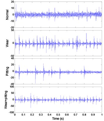
Fig. 1Signals and corresponding q-order RMS

As shown in Fig. 1, the -order local root mean square (qRMS, i.e., ) of fault bearing signal and normal bearing signal are calculated. With positive , are sensitive to the transient impulses in the signal (black dashed line). In contrast, with negative , are sensitive to local fluctuations with small magnitudes between adjacent impulses (purple dashed line). With and –2, are more sensitive to impulses and small local fluctuations than those with 1 and –1. When , is neutral to both of impulses and small local fluctuations.
The mono-fractal DFA method [12-14] () can only detect the transient impulses in a specific scale, which is insufficient to reveal the characteristics of the signals. In contrast, MFDFA can embody fractal characteristics of impulses and small local fluctuations in different scales, which can represent the operating status of rotating machinery more comprehensively.
For non-stationary rotating machinery vibration signals, there are significant nonlinear characteristics, especially in the range of transient impulse waveform. The local fluctuations depend on the fitting result of local trend. The fitting effects of fault bearing signal with different polynomial order are shown in Fig. 2. The cumulative series are divided into 3 regions according to waveform. The mean of local RMS in each region are shown in Table 1.
Fig. 2Local RMS with different polynomial order
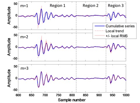
Table 1Mean of local RMS
Mean | |||
Region 1 | Region 2 | Region 3 | |
1 | 4.5312 | 0.5373 | 5.2732 |
2 | 2.6389 | 0.3553 | 2.4228 |
3 | 1.0233 | 0.2616 | 1.4997 |
4 | 0.5588 | 0.1928 | 1.0678 |
5 | 0.4610 | 0.1621 | 1.0584 |
When 1, the local trend are linear and the means of RMS in transient impulse regions 1 and 3 are much larger than those with higher polynomial orders. With the polynomial order increasing, the means of RMS are reduced significantly. When increases to 5, the RMS reduction becomes small.
Transient impulses are widespread in rotating machinery fault signals, similar but different fault patterns might contain similar transient impulses. Therefore, when linear local trend () is powerless to highlight the subtle differences among similar fault patterns, a higher polynomial order is necessary.
3. Multifractal manifold based on detrended fluctuation analysis
3.1. Multifractal feature based on DFA
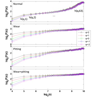
In multifractal spectrum [15], the generalized Hurst exponent are corresponding to the slopes of linear fitting line of - logarithmic curves with different order . Since the non-stationary characteristics of rotating machinery vibration signals, the logarithmic relationships between and are nonlinear and cannot be represented by the slopes of overall linear fitting line. Thereby, Moura [12, 13] selected with different as feature vector for each vibration signal and reduce the dimension of feature vectors with PCA to recognize signal patterns; Lin [14] used segmented slopes of logarithmic curves according to crossover characteristics to recognize signal patterns. The 2 methods are both based on mono-fractal DFA () and the features lack some nonlinear characteristics in varying degrees.
In order to represent the nonlinear characteristics of - logarithmic curves, the multifractal feature based on DFA can be defined as:
are the slopes of adjacent and in logarithmic curves. Where the segment length , [–2, –1, 0, 1, 2] and 1, 2,…, . Thereby, a matrix is obtained. The matrix can be converted to a multifractal feature vector () by connecting each row:
3.2. Manifold learning
The multifractal feature vectors are high-dimensional features with nonlinear characteristics. In order to recognize the patterns of high-dimensional nonlinear features, manifold learning [16, 17] is applied. Manifold learning is a global nonlinear dimensionality reduction method, which is mainly used in pattern and image recognition.
LTSA [18] is an effective manifold learning technique for nonlinear dimensionality reduction. For samples from different signal patterns, a multifractal feature matrix can be expressed as:
The feature dimension of multifractal feature matrix can be reduced to () by LTSA as following steps [18]:
(1) Extracting local information.
Determine the nearest neighborhoods for each vector through the Euclidean distance:
Centralize the matrix by removing the mean of corresponding nearest neighborhoods and then calculate the largest right singular vectors of the centralized matrix to obtain the orthogonal basis :
(2) Constructing alignment matrix.
Determine the 0-1 selection matrix :
Calculate the correlation matrix :
where is a column vector of ones.
Construct the alignment matrix :
(3) Aligning global coordinates.
Calculate the smallest eigenvectors of matrix , and then the 2nd to the th smallest eigenvalues are selected to constitute the global coordinates (). Thence, the -dimension multifractal manifold features can be expressed as:
where (1, 2,…, ) is corresponding to the th dimensionality reduction results.
The low-dimensional multifractal manifold features can reveal the differences of different signal patterns which are beneficial for pattern recognition and fault diagnosis.
Combining the advantages of MFDFA in time series nonlinear characteristics extraction and manifold learning in nonlinear dimensionality reduction, a novel multifractal manifold method is proposed. The proposed MFM method contains 3 steps:
(1) Calculate the fluctuation functions of series according to MFDFA with an appropriate polynomial order.
(2) Construct nonlinear multifractal feature vector for each signal series according to Eqs. (9-10).
(3) Reduce the dimension of multifractal feature vectors through manifold learning for pattern recognition.
4. Experimental verification
The proposed MFM method is tested by 4 cases of rotating machinery fault. For comparison, several related method are also tested. The corresponding methods are shown as follows:
(1) MFM: the proposed method, the low-dimensional features are MFMs.
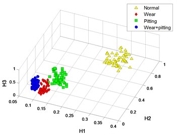
(2) Crossover characteristics [14]: the segmented slopes of - logarithmic curve based on mono-fractal DFA are applied to represent the characteristics of signal series, which are H1, H2 and H3 (polynomial order 1).
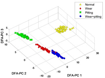
(3) DFA-PC [12, 13]: the mono-fractal fluctuation functions with different are selected as feature vectors to represent the characteristics of signal series, the dimension of vectors are reduced by PCA. The low-dimensional features are DFA-PCs (polynomial order ).
(4) MF-PC: based on DFA-PC method, the multifractal fluctuation functions are selected as feature vectors and the dimension of vectors are also reduced by PCA. The low-dimensional features are MF-PCs.
To test the performance of each method, clustering results of signal samples are obtained. 50 samples from each pattern are divided into two parts randomly: 20 train samples and 30 test samples, and then test samples are classified by support vector machine (SVM) [20, 21].
In all cases, the segment lengths are set to be [16, 32, 48,…, 1024] and the fluctuation function orders are set to be [–2, –1, 0, 1, 2].
4.1. Case I: Gearbox fault
The signal samples are acquired from a single cylindrical gear reducer. The signal patterns are normal, driven gear pitting, driving gear wear and mixed fault (driving gear wear and driven gear pitting). The sampling frequency is 5120 Hz. Each sample contains 5120 sampling points. The parameters of gears are shown in Table 2.
Table 2Gear parameters
Gear | Teeth | Rotating frequency (Hz) | Meshing frequency (Hz) |
Driving | 55 | 14.3 | 788 |
Driven | 75 | 10.5 | 788 |
The signal of each pattern is shown in Fig. 3(a). The multifractal - logarithmic curves and multifractal features are shown in Fig. 3(b) ().
Fig. 3a) Gearbox signals, b) multifractal logarithmic curves
a)
b)
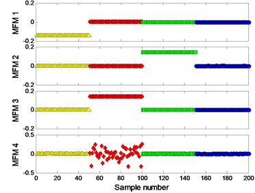
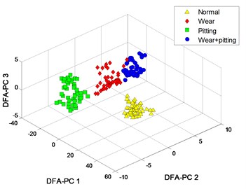
The clustering results of MFM and MF-PC with different polynomial order are shown in Fig. 4. The first 3 low-dimensional features of MFM () reveal the differences of signal samples, the samples from each pattern have the same features and all samples are distributed at 4 points, as shown in Fig. 4(a), (b); when , the samples from wear and mixed fault patterns are not completely distinguished, as shown in Fig. 4(c), (d). As shown in Fig. 4(e), (f), the signal samples are distinguished from each other by the first 3 low-dimensional features of MF-PC. However, the distribution variance of simples with is smaller than that with .
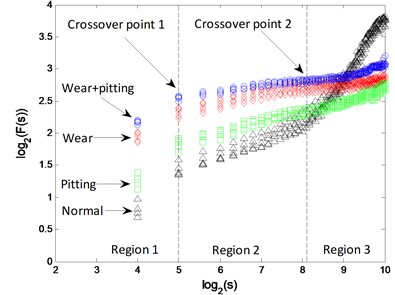
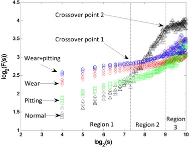
The - logarithmic curves based on mono-fractal DFA are calculated. For each signal pattern, the curves of 5 samples are plotted in Fig. 5. The curves are divided into 3 regions according to the crossover points and the slopes of fitting lines in each region are H1, H2 and H3.
The clustering results of crossover characteristics and DFA-PC are shown in Fig. 6. Most signal samples are distinguished from each other; only several samples are difficult to identify.
The classification results of SVM are shown in Table 3. All samples from different patterns are classified by 4 methods with high accuracies, while only MF-PC method and the MFM method with 3 classify samples completely correct.
Fig. 4Process results
a) MFM features with 3
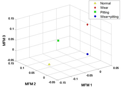
b) MFM with 3
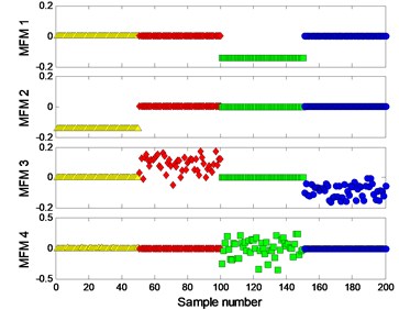
c) MFM features with 1
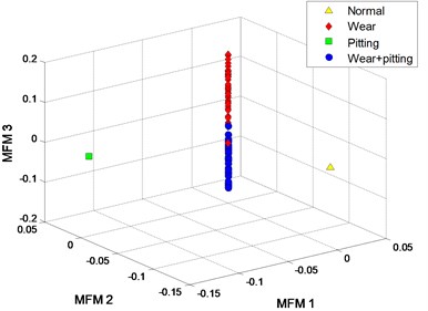
d) MFM with 1
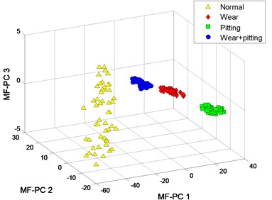
e) MF-PC with
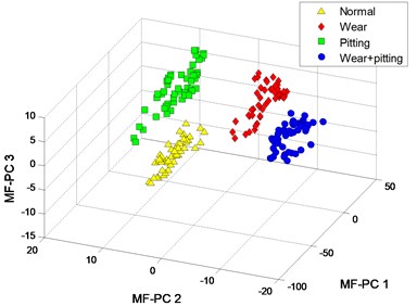
f) MF-PC with
Table 3Classification results
Method | Classification accuracy (%) | |||||
I | II | III | IV | mean | ||
MFM | 3 | 100 | 100 | 100 | 100 | 100 |
MFM | 1 | 100 | 93.33 | 100 | 100 | 98.33 |
Crossover | 3 | 100 | 100 | 96.67 | 100 | 99.17 |
Crossover | 1 | 100 | 96.67 | 100 | 100 | 99.17 |
DFA-PC | 3 | 100 | 93.33 | 100 | 100 | 98.33 |
DFA-PC | 1 | 100 | 93.33 | 100 | 100 | 98.33 |
MF-PC | 3 | 100 | 100 | 100 | 100 | 100 |
MF-PC | 1 | 100 | 100 | 100 | 100 | 100 |
Fig. 5Mono-fractal logarithmic curves of gearbox signals
a)
b)
Fig. 6Process results
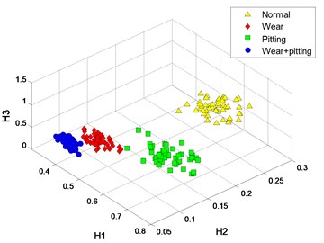
a) Crossover characteristics with 3
b) Crossover characteristics with 1
c) DFA-PC with 3
d) DFA-PC with 1
4.2. Case II: bearing rolling element with multi defect severities
Bearing data with different defect severities is obtained from the CWRU bearing data center [22]. All signal samples are acquired from normal bearing (type SKF-6205) and bearings with defects on the surface of rolling element and the defect sizes are 0.007, 0.014, 0.021 and 0.028 inch. The rotating speed of drive shaft is 1730 revolutions per minute (RPM) and the sampling frequency is 12000 Hz. Each sample contains 4800 sampling points.
The signal of each pattern is shown in Fig. 7(a). The multifractal logarithmic curves and multifractal features are shown in Fig. 7(b) ( 4).
Fig. 7Signals of bearings
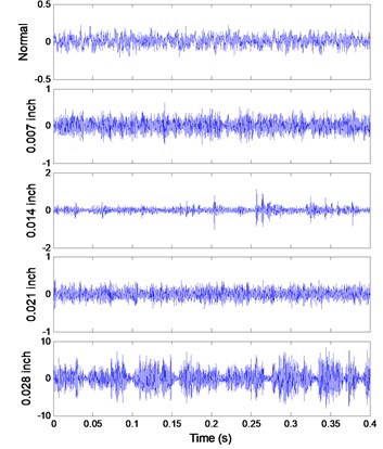
a) Signals
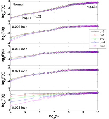
b) Multifractal logarithmic curves
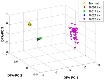
The clustering results of MFM and MF-PC are shown in Fig. 8. 4 MFM features ( 4) reveal the differences of signal samples; in order to represent these features in 3-dimension, 4 MFM features are reduced to 3 by PCA and the corresponding features are MFM-PCs, the samples from 5 patterns are distributed at 5 points, as shown in Fig. 8(a), (b); when , the samples from fault patterns of defect sizes 0.007 and 0.021 inch are recognized as a same pattern incorrectly, as shown in Fig. 8(c), (d). Simultaneously, the samples from fault patterns of defect sizes 0.007 and 0.021 inch patterns are still difficult to be distinguished by MF-PC method, as shown in Fig. 8(e), (f).
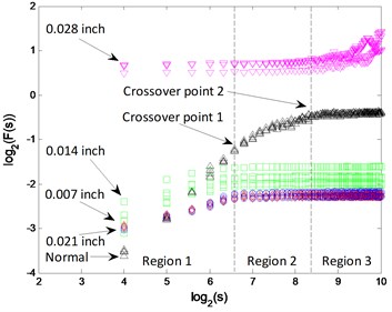
The - logarithmic curves based on mono-fractal DFA are calculated. For each signal pattern, the curves of 5 samples are plotted in Fig. 9. The curves are divided into 3 regions according to the crossover points and the slopes of fitting lines in each region are H1, H2 and H3.
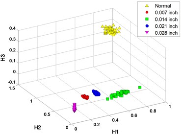
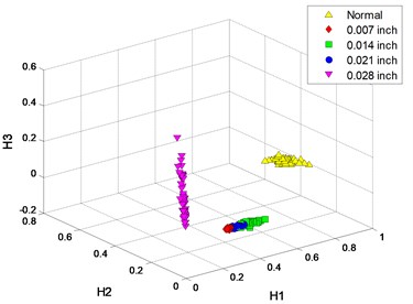
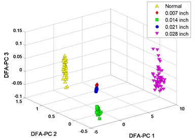
The clustering results of crossover characteristics and DFA-PC are shown in Fig. 10. 5 signal patterns are distinguished from each other with a higher polynomial order , as shown in Fig. 10(a), (c); while the samples from fault patterns of defect sizes 0.007 and 0.021 inch are unrecognizable when , as shown in Fig. 10(b), (d).
The classification results of SVM are shown in Table 4. When , there are different quantities of misclassified samples in the result of each method and the error samples are mainly from fault patterns of defect sizes 0.007 and 0.021 inch. With a higher polynomial order , the classification accuracies of all 4 methods are significantly improved.
Table 4Classification results
Method | Classification accuracy (%) | ||||||
I | II | III | IV | V | mean | ||
MFM | 4 | 100 | 100 | 100 | 100 | 100 | 100 |
MFM | 1 | 100 | 0 | 100 | 0 | 100 | 60 |
Crossover | 4 | 100 | 100 | 100 | 100 | 100 | 100 |
Crossover | 1 | 100 | 86.67 | 90 | 86.67 | 100 | 92.67 |
DFA-PC | 4 | 100 | 100 | 100 | 100 | 100 | 100 |
DFA-PC | 1 | 100 | 100 | 96.67 | 66.67 | 100 | 92.67 |
MF-PC | 4 | 100 | 93.33 | 100 | 100 | 100 | 98.67 |
MF-PC | 1 | 100 | 96.67 | 100 | 56.67 | 100 | 90.67 |
Fig. 8Process results
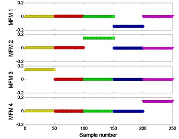
a) MFM features with 4
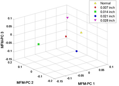
b) MFM with 4
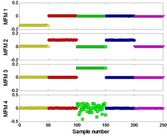
c) MFM features with 1
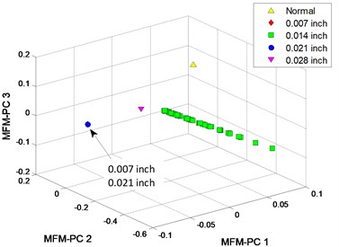
d) MFM with 1
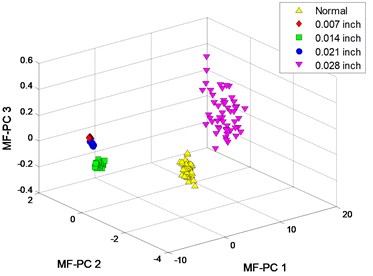
e) MF-PC with
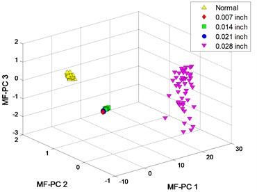
f) MF-PC with
Fig. 9Mono-fractal logarithmic curves of bearing signals
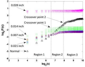
a) 4
b)
Fig. 10Process results
a) Crossover characteristics with 4
b) Crossover characteristics with 1
c) DFA-PC with 4
d) DFA-PC with 1
4.3. Case III: bearing consecutive extended defect
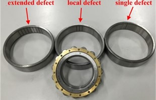
Self-aligning ball bearings (type HRB-1209) with different ranges of pitting defects and normal bearing are installed to the test end and tested individually, as shown in Fig. 11. The depths of artificially machined pitting defects are 0-0.5 mm. The rotating frequency of motor is 15 Hz and the signal sampling frequency is 25600 Hz. Each sample contains 12800 sampling points. The size ranges of bearing defects are shown in Table 5.
Table 5Parameters of bearings
Defect type | Defective range | Fault frequency (Hz) |
Normal | 0 | – |
Local defect | /16 | 102.5 |
Extended defect | 5/16 | 102.5 |
Fig. 11Experimental apparatus
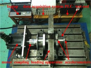
a) Experimental platform
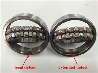
b) Bearings with defects
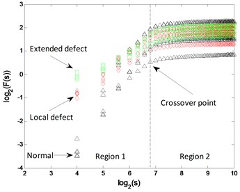
The signal of each pattern is shown in Fig. 12(a). The multifractal - logarithmic curves and multifractal features are shown in Fig. 12(b) ( 3).
Fig. 12Signals of bearings
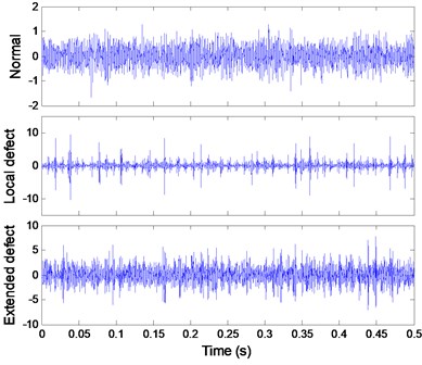
a) Signals
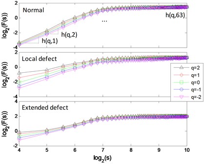
b) Multifractal logarithmic curves
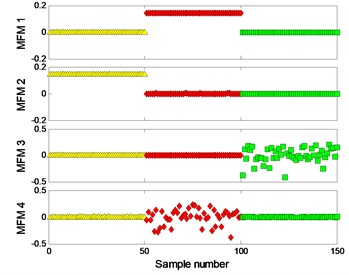
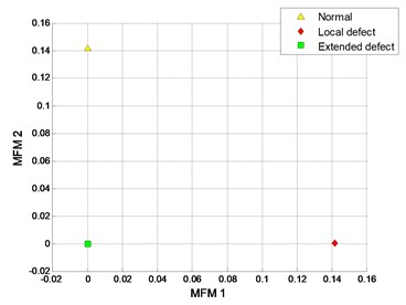
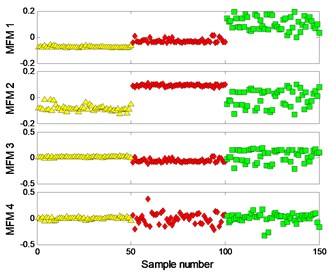
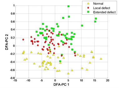
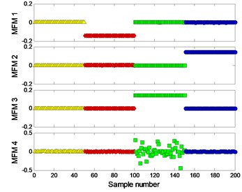
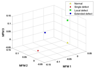
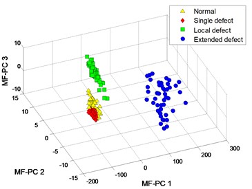
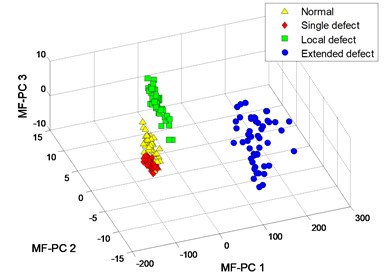
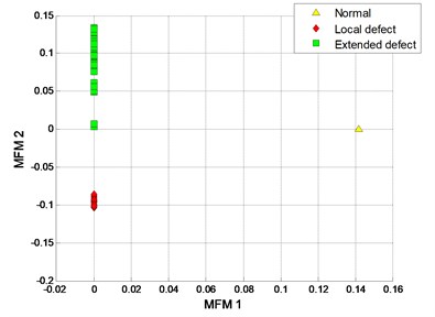
The clustering results of MFM and MF-PC are shown in Fig. 13. The first 2 low-dimensional features of MFM ( 3) reveal the differences of signal samples, the samples from each pattern have the same features and all samples are distributed at 3 points, as shown in Fig. 13(a), (b); when 1, the samples from local defect and extended defect fault patterns are not completely distinguished, as shown in Fig. 13(c), (d). The first 2 low-dimensional features of MF-PC are applied to identify the signal samples; the mixing phenomenon of samples is obvious, as shown in Fig. 13(e), (f).
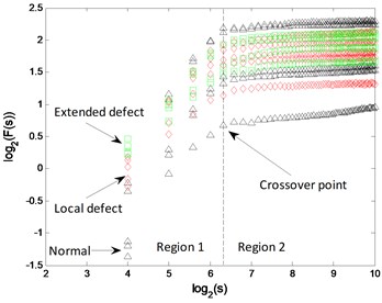
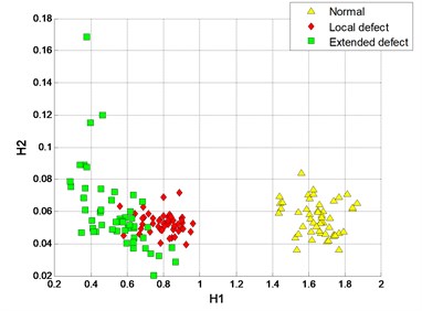
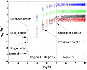
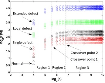
The logarithmic curves based on mono-fractal DFA are calculated. For each signal pattern, the curves of 5 samples are plotted in Fig. 14. The curves are divided into 2 regions according to the crossover point and the slopes of fitting lines in each region are H1 and H2.
The curves from 3 patterns are very similar in both of and segmented slopes. Therefore, the clustering results of the 2 methods based on DFA are unsatisfactory, as shown in Fig. 15.
The classification results of SVM are shown in Table 6. With a higher polynomial order, the classification accuracies are improved. The signal samples are correctly classified by the proposed MFM method; however, the signal samples are still hardly identified by the 2 DFA-based methods and MF-PC method.
Table 6Classification results
Method | Classification accuracy (%) | ||||
I | II | III | mean | ||
MFM | 3 | 100 | 100 | 100 | 100 |
MFM | 1 | 100 | 100 | 83.33 | 94.44 |
Crossover | 3 | 100 | 90 | 76.67 | 88.89 |
Crossover | 1 | 90 | 73.33 | 83.33 | 82.22 |
DFA-PC | 3 | 100 | 80 | 100 | 93.33 |
DFA-PC | 1 | 86.67 | 83.33 | 86.67 | 85.56 |
MF-PC | 3 | 96.67 | 96.67 | 86.67 | 93.33 |
MF-PC | 1 | 90 | 93.33 | 86.67 | 90 |
Fig. 13Process results
a) MFM features with 3
b) MFM with 3
c) MFM features with 1
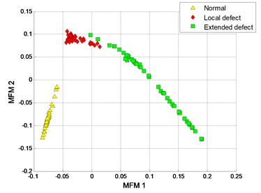
d) MFM with 1
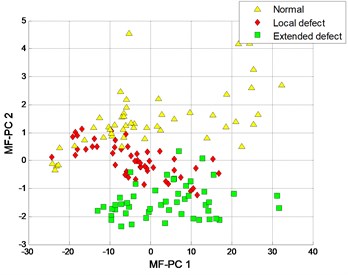
e) MF-PC with 3
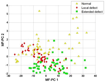
f) MF-PC with
Fig. 14Mono-fractal logarithmic curves of bearing signals
a)
b)
Fig. 15Process results
a) Crossover characteristics with 3
b) Crossover characteristics with 1
c) DFA-PC with 3
d) DFA-PC with 1
4.4. Case IV: bearing discrete extended defect
Cylindrical roller bearings (type TMB-N209M) with different number of defects and normal bearing are also tested on the experiment platform in Fig. 11(a). The sizes of artificially machined defects are 0.5 mm in depth and 0.6 mm in width. The rotating frequency of motor is 15 Hz and the signal sampling frequency is 25600 Hz. Each sample contains 12800 sampling points. The amount and feature of bearing defects are shown in Table 7 and Fig. 16.
Table 7Parameters of bearings
Defect type | Defects number | Fault frequency (Hz) |
Normal | 0 | – |
Single defect | 1 | 95.19 |
Local defect | 3 | 285.57 |
Extended defect | 9 | 285.57 |
Fig. 16Bearings with discrete defects
The signal of each pattern is shown in Fig. 17(a). The multifractal - logarithmic curves and multifractal features are shown in Fig. 17(b) ( 4).
Fig. 17Signals of bearings
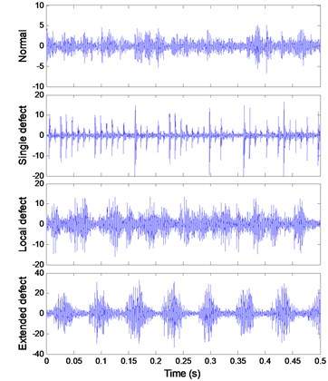
a) Signals
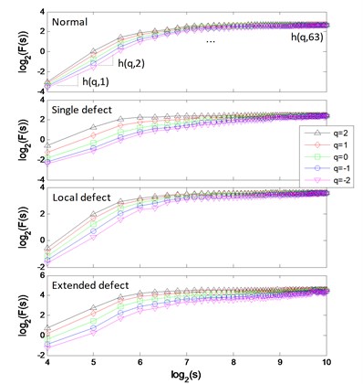
b) Multifractal logarithmic curves
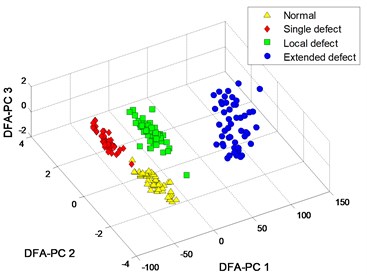
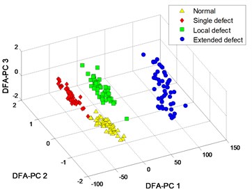
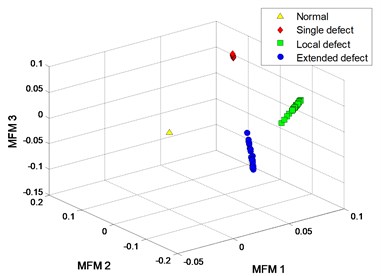
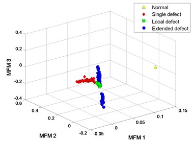
The clustering results of MFM and MF-PC are shown in Fig. 18. The first 3 low-dimensional features of MFM ( 4) reveal the differences of signal samples, the samples from each pattern have the same features and all samples are distributed at 4 points, as shown in Fig. 18(a), (b); when 1, the samples from 3 fault patterns are not distinguished from each other accurately, as shown in Fig. 18(c), (d). The clustering results of MF-PC with different polynomial orders are similar and the samples from normal and single defect patterns are mixed, as shown in Fig. 18(e), (f).
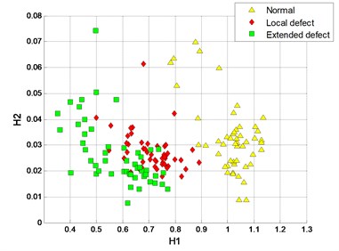
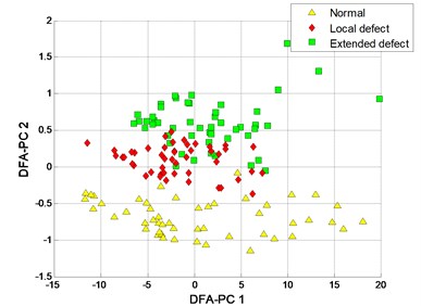
The - logarithmic curves based on mono-fractal DFA are calculated. For each signal pattern, the curves of 5 samples are plotted in Fig. 19. The curves are divided into 3 regions according to the crossover points and the slopes of fitting lines in each region are H1, H2 and H3.
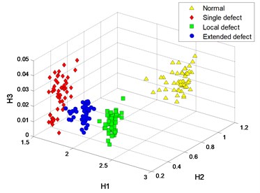
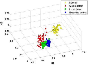
The segmented slopes of curves from 3 fault patterns are similar, and of samples from normal and single defect patterns are similar. Therefore, some samples from different patterns are mixed in the clustering results of the 2 DFA-based methods, as shown in Fig. 20.
The classification results of SVM are shown in Table 8. With a higher polynomial order, the classification accuracies are improved. The signal samples are correctly classified by the proposed MFM method; however, the misclassified samples still exist in the results of the 2 DFA-based methods and MF-PC method.
Table 8Classification results
Method | Classification accuracy (%) | |||||
I | II | III | IV | mean | ||
MFM | 4 | 100 | 100 | 100 | 100 | 100 |
MFM | 1 | 100 | 86.67 | 100 | 100 | 96.67 |
Crossover | 4 | 100 | 96.67 | 100 | 93.33 | 97.5 |
Crossover | 1 | 100 | 96.67 | 80 | 96.67 | 93.33 |
DFA-PC | 4 | 96.67 | 96.67 | 100 | 100 | 98.33 |
DFA-PC | 1 | 100 | 93.33 | 100 | 100 | 98.33 |
MF-PC | 4 | 86.67 | 96.66 | 100 | 100 | 95.83 |
MF-PC | 1 | 90 | 90 | 100 | 100 | 95 |
Fig. 18Process results
a) MFM features with 4
b) MFM with 4
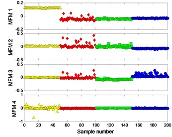
c) MFM features with 1
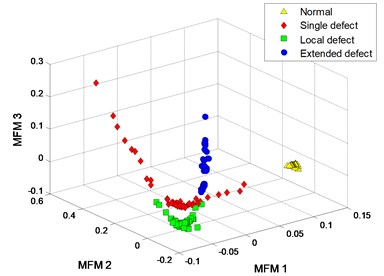
d) MFM with 1
e) MF-PC with 4
f) MF-PC with
Fig. 19Mono-fractal logarithmic curves of bearing signals
a)
b)
Fig. 20Process results
a) Crossover characteristics with 3
b) Crossover characteristics with 1
c) DFA-PC with 3
d) DFA-PC with 1
5. Discussions
For case III, the clustering results of MFM with 3 and 1 are shown in Fig. 13(b), (d), and the clustering result with 2 is shown in Fig. 21. For case IV, the clustering results of MFM with 4 and 1 are shown in Fig. 18(b), (d), and the clustering results with 3 and 2 are shown in Fig. 22(a), (b). The comparisons show that the mixed samples are gradually separated from each other with the increase of polynomial order. In 4 cases, the recognition performances of 4 methods are improved in varying degrees with higher polynomial orders.
Fig. 21MFM of case III with m= 2
As the mono-fractal logarithmic curves of case I shown in Fig. 5, the logarithmic curves of different patterns are easily identified and the DFA-based methods with linear polynomial order 1 have achieved high classification accuracies, therefore, the improvement of method based on multifractal DFA is not noticeable.
In case II, the classification results of 4 methods with high polynomial order are more accurate than those with polynomial order 1. While in case III and IV, the DFA-based methods [12-14] cannot identify the samples accurately since the and segmented slopes based on mono-fractal logarithmic curves are similar, as shown in Fig. 14 and Fig. 19; due to the nonlinear characteristics of high-dimensional features, even the multifractal theory is introduced into DFA-PC method the recognition performance of MF-PC method is not improved obviously compared to DFA-PC method [12, 13].
In 4 cases, the proposed MFM method with higher polynomial orders ( 2) has a superior performance in signal pattern recognition, which is benefit for rotating machinery fault diagnosis.
Fig. 22Process results of case IV
a) MFM with 3
b) MFM with 2
6. Conclusions
In this study, a multifractal manifold method based on detrended fluctuation analysis is proposed to reveal the nonlinear characteristics of vibration signals. The fault diagnosis performance of the MFM method is compared with other DFA-based methods and verified by fault experiments of gearbox and rolling element bearing. The experiment and verification results indicate that a higher polynomial order can improve the recognition results of signal patterns, which is ignored in DFA-based methods [12-14]. The low-dimensional MFM features can accurately represent the patterns of different signal samples, which are benefit for automatic pattern recognition and multiple fault diagnosis. The comparison results indicate that the MFM method can overcome the disadvantages of DFA-based methods and has a superior performance in signal pattern recognition.
References
-
Sheen Y. T., Hung C. K. Constructing a wavelet-based envelope function for vibration signal analysis. Mechanical Systems and Signal Processing, Vol. 18, Issue 1, 2004, p. 119-126.
-
Yan R., Gao R. X. Harmonic wavelet-based data filtering for enhanced machine defect identification. Journal of Sound and Vibration, Vol. 329, Issue 15, 2010, p. 3203-3217.
-
Ibrahim G., Albarbar A. Comparison between Wigner-Ville distribution and empirical mode decomposition vibration-based techniques for helical gearbox monitoring. Proceedings of the Institutuion of Mechanical Engineers Part C – Journal of Mechanical Engineering Science, Vol. 225, 2011, p. 1833-1846.
-
Li H., Zheng H., Tang L. Wigner-Ville distribution based on EMD for faults diagnosis of bearing. Fuzzy Systems and Knowledge Discovery, Vol. 4223, 2006, p. 803-812.
-
Antoni J. The spectral kurtosis: a useful tool for characterizing non-stationary signals. Mechanical Systems and Signal Processing, Vol. 20, Issue 2, 2006, p. 282-307.
-
Combet F., Gelman L. Optimal filtering of gear signals for early damage detection based on the spectral kurtosis. Mechanical Systems and Signal Processing, Vol. 23, Issue 3, 2009, p. 652-668.
-
Huang N. E., Shen Z., Long S. R. The empirical mode decomposition and Hilbert spectrum for nonlinear and non-stationary time series analysis. Proceedings of the Royal Society of London, Series A – Mathematical Physical and Engineering Sciences, Vol. 454, 1998, p. 903-995.
-
Lei Y., Lin J., He Z. A review on empirical mode decomposition in fault diagnosis of rotating machinery. Mechanical Systems and Signal Processing, Vol. 35, Issues 1-2, 2013, p. 108-126.
-
Zhang J., Yan R., Gao R. X. Performance enhancement of ensemble empirical mode decomposition. Mechanical Systems and Signal Processing, Vol. 24, Issue 7, 2010, p. 2104-2123.
-
Peng C. K., Havlin S., Stanley H. E. Quantification of scaling exponents and crossover phenomena in nonstationary heartbeat time series. Chaos, Vol. 5, 1995, p. 82-87.
-
Peng C. K., Buldyrev S. V., Havlin S. Mosaic organization of DNA nucleotides. Physical Review E, Vol. 49, Issue 2, 1994, p. 1685-1689.
-
Moura E. P., Vieira A. P., Irmão M. A. S. Applications of detrended-fluctuation analysis to gearbox fault diagnosis. Mechanical Systems and Signal Processing, Vol. 23, Issue 3, 2009, p. 682-689.
-
Moura E. P., Souto C. R., Silva A. A. Evaluation of principal component analysis and neural network performance for bearing fault diagnosis from vibration signal processed by RS and DF analyses. Mechanical Systems and Signal Processing, Vol. 25, Issue 5, 2011, p. 1765-1772.
-
Lin J., Chen Q. A novel method for feature extraction using crossover characteristics of nonlinear data and its application to fault diagnosis of rotary machinery. Mechanical Systems and Signal Processing, Vol. 48, Issues 1-2, 2014, p. 174-187.
-
Kantelhardt J. W., Zschiegner S. A., Koscielny-Bunde E. Multifractal detrended fluctuation analysis of nonstationary time series. Physica A – Statistical Mechanics and Its Applications, Vol. 316, Issues 1-4, 2002, p. 87-114.
-
Tenenbaum J. B., Silva V., Langford J. C. A global geometric framework for nonlinear dimensionality reduction. Science, Vol. 290, Issue 5500, 2000, p. 2319-2323.
-
Roweis S. T., Saul L. K. Nonlinear dimensionality reduction by locally linear embedding. Science, Vol. 290, Issue 5500, 2000, p. 2323-2326.
-
Zhang Z. Y., Zha H. Y. Principal manifolds and nonlinear dimensionality reduction via tangent space alignment. SIAM Journal on Scientific Computing, Vol. 26, Issue 1, 2004, p. 313-338.
-
Kantelhardt J. W., Koscielny-Bunde E., A. Rego H. H. Detecting long-range correlations with detrended fluctuation analysis. Physica A, Vol. 295, Issues 3-4, 2001, p. 441-454.
-
Widodo A., Yang B. S. Support vector machine in machine condition monitoring and fault diagnosis. Mechanical Systems and Signal Processing, Vol. 21, Issue 6, 2007, p. 2560-2574.
-
Hsu C. W., Lin C. J. A comparison of methods for multiclass support vector machines. IEEE Transactions on Neural Networks, Vol. 13, Issue 2, 2002, p. 415-425.
-
http://csegroups.case.edu/bearingdatacenter/pages/download-data-file.
Cited by
About this article

This work is supported by the National Natural Science Foundation of China (Nos. 51275245 and 61374133).
