Parallel simulation based adaptive prediction for equipment remaining useful life

Ge, Chenglong; Zhu, Yuanchang; Di, Yanqiang; Dong, Zhihua

doi:10.21595/jve.2018.18973

Journal of Vibroengineering

Browse Journal

Submit article

Published: 15 August 2018

Check for updates

Parallel simulation based adaptive prediction for equipment remaining useful life

Chenglong Ge¹

Yuanchang Zhu²

Yanqiang Di³

Zhihua Dong⁴

^{1, 2, 3}Mechanical Engineering College, Shijiazhuang, P. R. China

⁴Baicheng Ordnance Test Center, Baicheng, P. R. China

Corresponding Author:

Chenglong Ge

Cite the article Download PDF

Downloads 1753

WoS Core Citations 1

CrossRef Citations 1

Abstract

The latest demands for remaining useful life (RUL) prediction are online prediction, real-time prediction and adaptive prediction. This paper addresses the demands of RUL prediction and proposes a novel framework of parallel simulation based adaptive prediction for equipment RUL. In the framework, a Wiener state space model (WSSM) is developed to achieve the aim, which considers the whole historical data and monitoring noise. Driven by the online observation data, the degradation state is estimated by the Kalman filter based data assimilation and the WSSM parameters are updated by the expectation maximum algorithm. An analytical RUL distribution considering the distribution of the degradation state is obtained based on the concept of the first hitting time. A case study for GaAs laser device is provided to substantiate the superiority of the proposed method compared with the competing method of traditional Wiener process. The results show that the parallel simulation method can provide better RUL prognostic accuracy.

1. Introduction

In the field of equipment maintenance support, the PHM is an important means to achieve equipment accurate maintenance [1]. The PHM can execute reasonable maintenance and management to ensure the safety, economy and reliability of equipment operation by predicting the remaining useful life of the equipment accurately. The key technologies of PHM include RUL forecasting and health management, and the RUL prognosis is the core content of PHM [2]. RUL is defined as the time length from the current time to the failure moment [3] what is the important basis and basic premise for maintenance decision.

The commonly used RUL prediction models include the random coefficient regression model [4], gray model [5], neural network model [6], similarity model [7], hidden Markov model [8], support vector machine model [9] and random process model, etc. However, these models have the following deficiencies. Firstly, most of the models can only be used offline, i.e., for online monitoring and offline prediction. The corresponding degradation data is obtained by online monitoring equipment and the remaining useful life is predicted through offline feature extraction. Its essence still belongs to the offline forecasting method with weak online prediction ability [10]. Secondly, the equipment requiring high safety urgently needs to acquire the remaining useful life in real time owing to the complexity of the equipment operating environment. However, the real-time prediction capability of the above models is weak. The real-time prediction problem mainly focuses on the calculation of the analytical expression for RUL probability density function [11]. Thirdly, most of the models belong to the static model without the dynamic adjustment ability. The model parameters are obtained from the historical data of the same type equipment by offline estimation such as maximum likelihood estimation. The dynamic adjustment problem focuses on the adaptive adjustment of the model parameters. Moreover, it is a difficult problem in the current research of RUL prediction to study the prognostic models with adaptive ability [12]. To sum up, the latest demands for RUL prediction are online prediction, real-time prediction and adaptive prediction.

In particular, a random process model of the Wiener process has a clear physical interpretation and good mathematical properties which has been widely used in degradation modeling and RUL prediction in recent years. For the first time, Doksum [13] applied the Wiener process to the accelerated degradation modeling and transformed the non-stationary Wiener process into the stationary Wiener process through time-scale transformation and then inferred the equipment lifetime at normal stress levels. Whitmore [14] characterized the accelerated degeneration data by using the Wiener process with time-scale transformation. Si [15] converted the general nonlinear degradation process into a standard Brownian motion and then derived an approximate first hitting time (FHT). The above studies were all based on the assumption that the degradation state can be directly observed. However, most equipment cannot satisfy this assumption. Therefore, it is necessary to treat the degradation state as a hidden state. So, Whitmore [16] used a Wiener process model with measurement noise to characterize the declining trend of transistor gain. Peng [17] used a Wiener process model with measurement noise and random drift coefficient to estimate the laser mean-time-to-failure (MTTF). It is notable that the linear Wiener process is actually a first-order Markov chain. In other words, the predicted degradation degree is only related to the current degradation degree rather than the whole historical data. As a result, this leads to the increase of prediction error. Therefore, on the basis of the linear Wiener process, Wang [1] first introduced the adaptive drift coefficient and used the Kalman filter to estimate the degradation state by utilizing the whole historical data. Further, Si [18] proposed an iterative degradation model based on the linear Wiener process, which took the uncertainty of the drift state into account and reduced the prediction uncertainty. Although there were many researches on equipment RUL prediction based on the linear Wiener process, few researchers predicted the RUL by considering the measurement noise and the whole historical data simultaneously. If both the measurement noise and the whole historical data could be taken into consideration, the accuracy and rationality of RUL prediction would be improved.

Therefore, it is urgent to provide a new means of RUL prediction which improves the prediction accuracy and meets the latest prediction demands. Equipment parallel simulation is a new emerging simulation technology in the field of system modeling and simulation. It has become a research emphasis which provides a completely new theory and method to solve the RUL prediction problem. The parallel simulation method uses the linear Wiener process to execute degradation modeling and establishes a Wiener state space model (WSSM). The WSSM takes the influence of measurement noise and historical data into account, what is beneficial to improve the prediction accuracy of RUL. On the basis of degradation modeling, the parallel simulation based equipment RUL prediction framework is proposed. The framework receives the equipment degradation data online and uses the Kalman filter and expectation maximization algorithm to drive the WSSM evolution dynamically. Then the distribution of the hidden degradation state is obtained and integrated into the inverse Gaussian distribution. Eventually, the analytic expression of RUL probability density function is achieved. In short, the framework realizes the online prediction, real-time prediction and adaptive prediction of RUL.

2. Equipment parallel simulation paradigm

2.1. Concepts and characteristics

Equipment parallel simulation is an emerging technology in the field of system modeling and simulation and has become a research emphasis. The concept and technical characteristics of parallel simulation are put forward in literature [19]. As a new simulation application paradigm, the equipment parallel simulation is designed to run the simulation system and weapon equipment through interaction. The simulation system obtains the weapon equipment information in real time to update the simulation model online. The weapon equipment, on the other hand, may benefit from the effects of feedback provided by the simulation system to improve equipment performance. The simulation system operated in this mode is called as a parallel simulation system. The word “parallel” of equipment parallel simulation is fundamentally different from “parallel” of parallel computing. The former refers to the fact that the complex problem is extended to a problem between the actual system and the virtual/simulation system which is dealt in an interactive way [20, 21]. But the latter refers to the fact that the complex problem is divided into sub-problems which are dealt at the same time [22].

Compared with the previous simulation technology, the equipment parallel simulation has the characteristics of symbiosis, two-way interaction, model evolution, data driven and efficient operation [23, 24]. Among them, model evolution is considered to be the core connotation and main technical characteristics of parallel simulation. The model construction in parallel simulation belongs to the category of evolutional modeling, including model parameter evolution and model output updating. The simulation system utilizes the equipment running data to evolve model parameters and to update the model output. As a result, the future state of the equipment can be evaluated or predicted based on the evolutionary simulation model. The simulation output may be closed to the actual state of equipment on the basis of model evolution, and the predictive accuracy of simulation system is improved finally.

2.2. Weapon equipment and parallel simulation system

The overview of equipment parallel simulation is shown in Fig. 1. In an equipment parallel simulation application, the weapon equipment is coupled with a parallel simulation system by sensors and actuators. The sensors provide information about the weapon equipment and the actuators allow the parallel simulation system controlling the weapon equipment. The simulation model of parallel simulation emphasizes dynamic evolution, adaptive updating and infinite approximation, which belongs to the category of simulation model set. The simulation model set includes simulation models obtained by different modeling methods and the corresponding model mirror images at a different time.

Fig. 1Overview of equipment parallel simulation

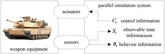
The information provided by sensors can be further distinguished between two types of information, i.e., information about the state $S_{t}$ and behavior $B_{t}$ of the weapon equipment at time $t$ . $S_{t}$ reflects the values of various internal state variables of the weapon equipment at any specific time. $B_{t}$ reflects quantifiable information about the weapon equipment that is not reflected by the state information. In the parallel simulation based adaptive prediction for equipment RUL, the state information $S_{t}$ is mainly concerned. The weapon equipment can be controlled by receiving the corresponding discrete control information $C_{t}$ at time $t$ . Because the acquisition of control information needs to be calculated or reasoned by the parallel simulation system for a certain period of time, it is considered as discrete control information. The control information may only be valid for a limited period of time or invalidated by control information $C_{t + 1}$ which is propagated to the weapon equipment at some later time $t + 1$ . In the parallel simulation based adaptive prediction for equipment RUL, the RUL and its probability density function (PDF) are the feedback of parallel simulation system, and they contain all hidden control information which is not included in $C_{t}$ . Based on the feedback results and maintenance experience, equipment maintenance personnel makes maintenance decision and then uses the actuators to perform maintenance manipulation, e.g., repair, replacement and other maintenance activities. PDF reflects the uncertainty of the RUL prediction, which is the primary prediction quantity. This paper focuses on the evolutionary modeling of parallel simulation based adaptive prediction for the equipment RUL.

3. Evolutionary modeling framework for parallel simulation

3.1. Evolutionary modeling analysis

In literature [25], it is pointed out that the performance degradation is the main cause of equipment failure, so the performance degradation based modeling is the preferred modeling direction of parallel simulation based adaptive prediction for the equipment RUL. The essence of RUL prediction is the estimation of equipment degradation state. Considering the dynamic change and implicitness of equipment degradation state, it is necessary to establish a state space model (SSM) of equipment degradation, including the degradation state evolution equation and the observation equation. Meanwhile, the impacts of the operating environment and the internal structure on the equipment performance degradation have the characteristics of randomness and uncertainty, so it is a reasonable choice to use a stochastic process model to explain the equipment degradation process. The equipment performance degradation modeling based on the stochastic process can describe the trend of equipment degradation by fitting the change trace of a performance degradation variable, and then it predicts the time interval from the present time to the time when the stochastic process reaches the failure threshold. The representative stochastic process is the Wiener process. Consequently, the construction of equipment degradation SSM based on the SSM and Wiener process is not only conducive to estimate the equipment degradation state but it is also helpful for describing the degradation process.

Data assimilation (DA) and parameters online estimation are the main technical means to realize the WSSM evolution. Due to the dynamic injection of the degraded data, the parallel simulation system should have the data assimilation ability to improve the adaptability and prediction ability of the simulation system. Data assimilation can reduce the influence of WSSM noise by importing the latest observation data into the WSSM, and the WSSM prediction trace is closer to the real degradation state by constantly correcting the WSSM output results. The commonly used data assimilation algorithms include Kalman filter (KF) [26] and particle filter (PF). The online parameter estimation algorithm is used to evolve the unknown parameters of WSSM, and the expectation maximum (EM) algorithm is the commonly used algorithm for estimating unknown parameters of SSM.

3.2. Framework of parallel simulation based adaptive prediction for equipment RUL

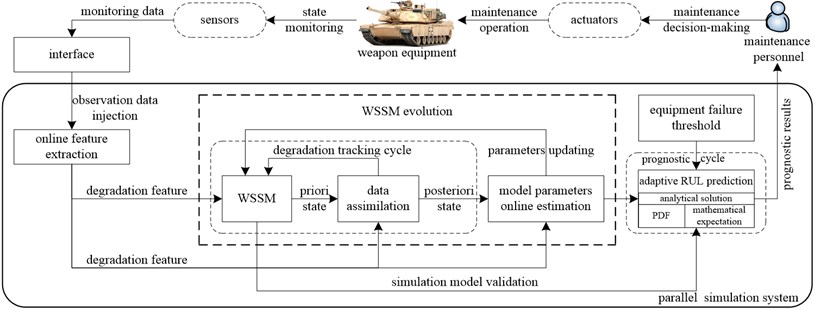
According to the above modeling analysis, the diagram of parallel simulation based adaptive prediction for equipment RUL is shown in Fig. 2. The framework has the following advantages. Firstly, it is an online prediction framework. The parallel simulation system can online receive the data provided by the sensors. Then the online processing and feature extraction for the observation data are implemented and the degradation feature is obtained. The prognostic results can be fed back to the equipment maintenance personnel online to support maintenance decision-making. Secondly, it is an adaptive prediction framework. The framework utilizes the KF based data assimilation algorithm to achieve the assimilation between the degradation state and the observation data, i.e., the WSSM output is updated. Simultaneously, the EM algorithm is used to adjust the WSSM parameters dynamically. Through the iteration of two algorithms, the WSSM parameters and output are updated adaptively, to provide the adaptive RUL prediction with the accurate model and the distribution of degradation state. In addition, it is a real-time prediction framework. Wiener SSM is regarded as the basic simulation model, and the FHT distribution of Wiener process is the inverse Gaussian distribution. With this excellent property, the distribution of degradation state can be integrated into the inverse Gaussian distribution. As a result, the analytical expression of the RUL’s PDF and RUL’s mathematical expectation are achieved. In other words, the real-time prediction is realized. The novel framework mainly includes the following steps:

Step 1: The degradation state of weapon equipment is monitored in real time by sensors such as vibration sensors, temperature sensors and other monitoring equipment, and the monitoring data is acquired.

Step 2: The monitoring data is transmitted to the parallel simulation system via the interface, and the equipment degradation state is sensed online by the parallel simulation system, which mainly involves the data preprocessing technology such as data noise reduction, missing data processing and abnormal data processing. Finally, the features which reflect the degradation state are obtained.

Step 3: Data assimilation between the real-time degraded feature and WSSM output is executed continuously based on the KF algorithm, and the tracking cycle of the equipment degradation state is realized. Moreover, the EM algorithm is used to estimate the unknown parameters of WSSM, and the evolution of the model parameters is accomplished to approach the equipment actual degradation state.

Step 4: Based on the implied degradation state obtained by parallel simulation and the equipment failure threshold, the equipment RUL and its PDF are predicted adaptively in real time.

Step 5: The prognostic results of parallel simulation system are taken as a feedback to transmit to the equipment personnel. According to the maintenance principles (e.g., safety, economy and mission) and maintenance experience, the maintenance scheme is developed by the equipment personnel.

Step 6: The actuators (e.g., equipment personnel, automatic maintenance equipment) are utilized to execute maintenance operations such as replacement of spare parts based on the maintenance scheme, and then the equipment support efficiency is improved.

Fig. 2Framework of parallel simulation based adaptive prediction for equipment RUL

Further, the parallel simulation method is discussed deeply from the following two aspects.

(1) Parallel simulation is a simulation method driven by the dynamic degradation data of the equipment. There was no data driven problem in the past simulation technology. On the contrary, the parallel simulation utilizes the dynamic data of the physical system to drive the simulation model evolution. In this paper, the Wiener state space model, which includes state equation and observation equation, is constructed. The essence of state equation is a linear Wiener process based simulation model of performance degradation and the observation equation establishes the relationship between the simulation output and the observed data. Then the WSSM is evolved driven by the degradation data. Specifically, the WSSM parameters are adjusted adaptively, and the WSSM output is updated. As a result, more accurate parameters and more accurate distribution of degradation state are used to predict the remaining useful life, and the RUL prognostic accuracy is improved.

(2) Parallel simulation is a simulation method with a feedback applied in the field of real-time decision support. There also were no the issues of the feedback of simulation results and the effects of feedback on the physical system. But in the parallel simulation based adaptive RUL prediction, the simulation results can be fed back to the equipment maintenance personnel. According to the simulation results, the maintenance scheme is developed by combining the maintenance principles with maintenance experience. Then the actuators are utilized to execute maintenance operation such as replacement of spare parts based on the maintenance scheme, i.e., the equipment operation is affected by the simulation results.

3.3. Equipment performance degradation modeling based on WSSM

3.3.1. Wiener process and offline MLE-IG method

The Wiener process is written as:

1

x (t) = x (0) + η t + σ B (t),

where $x (0)$ is the initial degradation state which is given with 0 in general, $η$ is the drift coefficient, and $σ$ is the diffusion coefficient. $B (t)$ is the standard Brownian motion and $B (t) ~ N (0, t)$ . Let us suppose that the equipment failure threshold is $ω$ , and the RUL of the equipment is $T$ , $T$ can be defined as the first hitting time of the standard Brownian motion crossing $ω$ , that is:

2

T (ω) = i n f \{t : x (t) \geq ω| x (0) < ω\} .

The mathematical expectation of the Wiener process is $E (x (t)) = η t$ which is a linear function of time $t$ , and the drift coefficient $η$ is an important parameter which reflects the degradation process. The variance of Wiener process is $v a r (x (t)) = σ^{2} t$ which represents the uncertainty of the degradation process at time $t$ . The real-time estimation of $η$ and $σ^{2}$ is the basis to realize the RUL prognosis accurately. Due to that the mathematical expectation of Wiener process is a linear function of time $t$ , the Wiener process is adapted to describe the linear degradation process. In the past method, the offline maximum likelihood estimation (MLE) was used to estimate the parameters of $η$ and $σ^{2}$ . Assuming that $g$ samples of performance degradation data can be obtained, then the degradation quantity of sample $i$ at the initial time $t_{i 0}$ is zero, i.e., $x_{i 0} = 0$ . The degradation data $x_{i 1}, \dots, x_{i m_{i}}$ is obtained by monitoring the degradation state at time $t_{i 1}, \dots, t_{i m_{i}}$ . Note that $Δ x_{i j} = x_{i j} - x_{i (j - 1)}$ is the degradation quantity between time $x_{i (j - 1)}$ and $x_{i j}$ . And according to the property of Wiener process:

3

Δ x_{i j} ~ (η Δ t_{i j}, σ^{2} Δ t_{i j}),

where $Δ t_{i j} = t_{i j} - t_{i (j - 1)}$ , $i = 1,2, \dots, g$ , $j = 1,2, \dots, m_{i}$ .

The PDF of $Δ x_{i j}$ is:

4

f (Δ x_{i j}; η Δ t_{i j}, σ^{2} Δ t_{i j}) = \frac{1}{\sqrt{2 π σ^{2} Δ t_{i j}}} e x p (- \frac{(Δ x_{i j} - η Δ t_{i j})^{2}}{2 σ^{2} Δ t_{i j}}) .

The likelihood function of $f (Δ x_{i j}; η Δ t_{i j}, σ^{2} Δ t_{i j})$ is:

5

L (η, σ^{2}) = \prod_{i = 1}^{g} \prod_{j = 1}^{m_{i}} f (Δ x_{i j}; η Δ t_{i j}, σ^{2} Δ t_{i j}) = \prod_{i = 1}^{g} \prod_{j = 1}^{m_{i}} \frac{1}{\sqrt{2 π σ^{2} Δ t_{i j}}} e x p (- \frac{(Δ x_{i j} - η Δ t_{i j})^{2}}{2 σ^{2} Δ t_{i j}}) .

The partial derivative of $L (η, σ^{2})$ is ordered into 0 against $η$ and $σ^{2}$ relatively, i.e.:

6

\{\begin{array}{l} \frac{\partial L (η, σ^{2})}{\partial η} = 0, \\ \frac{\partial L (η, σ^{2})}{\partial σ^{2}} = 0 . \end{array}

The maximum likelihood estimation of $η$ and $σ^{2}$ can be derived by:

7

\hat{η} = \frac{\sum_{i = 1}^{g} x_{i m_{i}}}{\sum_{i = 1}^{g} t_{i m_{i}}}, {\hat{σ}}^{2} = \frac{1}{\sum_{i = 1}^{g} m_{i}} (\sum_{i = 1}^{g} \sum_{j = 1}^{m_{i}} \frac{(Δ x_{i j})^{2}}{Δ t_{i j}} - \frac{{(\sum_{i = 1}^{g} x_{i m_{i}})}^{2}}{\sum_{i = 1}^{g} t_{i m_{i}}}) .

The FHT distribution of Wiener process is the inverse Gaussian (IG) distribution. So if $x (t_{i})$ is the degradation quantity of the equipment at time $t_{i}$ , the PDF of RUL are obtained, i.e.:

8

f (t) = \frac{ω - x (t_{i})}{\sqrt{2 π {\hat{σ}}^{2} t^{3}}} e x p (- \frac{(ω - x (t_{i}) - \hat{η} t)^{2}}{2 {\hat{σ}}^{2} t}) .

This traditional method is called as the offline MLE-IG method. Note that the offline MLE-IG method cannot realize the model evolution, and the method also neglects the impacts of historical data and monitoring noise on RUL. As a result, the prognostic results of RUL are inaccurate, and the larger prognostic error is inevitable to occur.

3.3.2. WSSM

For the construction of WSSM, the Euler discretization is first performed, and the evolution equation of the degradation state can be obtained, i.e.:

9

x_{k} = x_{k - 1} + η τ_{k} + σ B (τ_{k}) .

Owing to the influences of sensor accuracy and equipment operating conditions, the accurate degradation data cannot be directly measured. So considering the impact of measurement noise, the observation equation can be written as:

10

y_{k} = x_{k} + π_{k},

where $π_{k} ~ N (0, ϕ^{2})$ and $ϕ^{2}$ is the variance of monitoring noise. $π_{k}$ and $B (τ_{k})$ are assumed to be independent of each other. Eventually, the Wiener state space model is written as:

11

\{\begin{array}{l} x_{k} = x_{k - 1} + η τ_{k} + σ B (τ_{k}), \\ y_{k} = x_{k} + π_{k}, \end{array}

where $τ_{k} = t_{k} - t_{k - 1}$ is the sampling period. Moreover, the function of simulation is introduced from the following three aspects.

1) Providing the distribution of degradation state for RUL prediction. The degradation state is regarded as a hidden state in the WSSM. In other words, the simulation output $x_{k}$ is a hidden state. Meanwhile, the modeling method of state space can use the data assimilation mechanism, and then can obtain the distribution of degradation state.

2) Improving the RUL prognostic accuracy by considering the effects of monitoring noise and historical data. The observation equation of WSSM includes the monitoring noise which cannot be ignored in the RUL prediction. Furthermore, the parallel simulation method overcomes the influence of the Markov property by considering the historical data, which improves the RUL prognostic rationality. So, the RUL prognostic accuracy is more consistent with the actual RUL.

3) Improving the RUL prognostic accuracy by simulation model evolution. The drift coefficient $η$ and the diffusion coefficient $σ$ are the important parameters of WSSM. The accuracy of $η$ and $σ$ directly affects the probability density distribution of RUL. The parallel simulation method utilizes the Kalman filter and expectation maximization algorithm to adjust the model parameters and model output dynamically. As a result, the simulation results constantly approach the actual degradation state, and the RUL prognostic accuracy is improved.

4. WSSM evolution

4.1. Kalman filter based WSSM output updating

In this paper, the KF algorithm which can obtain the degradation state optimal estimation under the condition of the degradation state follows a linear change and the error follows the Gaussian distribution is used to realize the data assimilation. The essence of KF algorithm is to track the equipment degradation state. Using the KF algorithm to achieve the WSSM output correction mainly includes the prognostic stage and updating stage.

(1) Prognostic stage. The priori estimate ${\hat{x}}_{k | k - 1}$ and the covariance $P_{k | k - 1}$ of the degradation state $x_{k}$ at time $k$ are acquired by utilizing the posteriori estimate ${\hat{x}}_{k - 1 | k - 1}$ and the covariance $P_{k - 1 | k - 1}$ of the degradation state $x_{k - 1}$ at time $k - 1$ , that is:

12

{\hat{x}}_{k | k - 1} = {\hat{x}}_{k - 1 | k - 1} + η τ_{k},

13

P_{k | k - 1} = P_{k - 1 | k - 1} + σ^{2} τ_{k},

where:

14

P_{k - 1 | k - 1} = c o v (x_{k - 1}) = E [(x_{k - 1 | k - 1} - {\hat{x}}_{k - 1 | k - 1}) (x_{k - 1 | k - 1} - {\hat{x}}_{k - 1 | k - 1})^{T}] .

(2) Updating stage. The posteriori estimate of the degradation state $x_{k}$ is obtained by utilizing the observation value $y_{k}$ and priori estimate ${\hat{x}}_{k | k - 1}$ and the covariance $P_{k | k - 1}$ at time $k$ , that is:

15

{\tilde{y}}_{k} = y_{k} - {\hat{x}}_{k | k - 1},

16

S_{k} = P_{k | k - 1} + ϕ^{2},

17

K_{k} = P_{k | k - 1} {S_{k}}^{- 1},

18

{\hat{x}}_{k | k} = {\hat{x}}_{k | k - 1} + K_{k} {\tilde{y}}_{k},

19

P_{k | k} = (I - K_{k}) P_{k | k - 1},

where ${\tilde{y}}_{k}$ is the new information, $S_{k}$ is the variance of ${\tilde{y}}_{k}$ , $K_{k}$ is the Kalman gain, ${\hat{x}}_{k | k}$ and $P_{k | k}$ are the mean value and variance of $x_{k}$ at time $k$ respectively. Once the observation value is acquired, the posteriori estimate of the degradation state at time $k + 1$ can be obtained according to the Eqs. (12-19).

4.2. EM algorithm based WSSM parameters evolution

The unknown parameter set in the WSSM is defined as $θ = {η, σ, ϕ}$ which reflects the equipment degradation characteristics. The MLE-IG method uses different individual degradation data from the same type equipment to estimate parameters offline and as a result, the differences between individuals and the random effects of the operating environment are not taken into consideration. So, the prognostic accuracy will be improved if the parameters are estimated online according to the equipment real-time degradation data. The EM algorithm is an iterative algorithm which can effectively estimate the parameters of the SSM with a hidden state. The parallel simulation system can use the EM algorithm to perform online estimation of unknown parameters of WSSM in real time. The hidden states and the historical observation data are expressed as $X_{k} = {x_{1}, x_{2}, \dots, x_{k}}$ and $Y_{k} = {y_{1}, y_{2}, \dots, y_{k}}$ respectively.

At time $k$ , the estimation of $θ$ at the $l$ th iterative step of the EM algorithm, i.e., ${\hat{θ}}_{k}^{(l)}$ , can be given by:

20

{\hat{θ}}_{k}^{(l)} = a r g \underset{θ}{m a x} ψ (θ| {\hat{θ}}_{k}^{(l - 1)}) = a r g \underset{θ}{m a x} E_{X_{k} | Y_{k}, {\hat{θ}}_{k}^{(l - 1)}} φ_{k} (θ),

where $φ_{k} (θ)$ is the joint logarithm likelihood function of $X_{k}$ and $Y_{k}$ . $ψ (θ| {\hat{θ}}_{k}^{(l - 1)})$ denotes the mathematical expectation of $φ_{k} (θ)$ conditional on $Y_{k}$ and ${\hat{θ}}_{k}^{(l - 1)}$ . Eq. (20) can be divided into E-step and M-step.

4.2.1. E-step

The joint logarithm likelihood function of $X_{k}$ and $Y_{k}$ is calculated at first. According to WSSM, it can be known that $x_{i} | x_{i - 1} ~ N (x_{i - 1} + η τ, σ^{2} τ)$ and $y_{i} | x_{i} ~ N (x_{i}, ϕ^{2})$ . $φ_{k} (θ)$ can be formulated as:

21

φ_{k} (θ) = l n p (X_{k}, Y_{k}| θ),

φ_{k} (θ) = l n (\prod_{i = 1}^{k} p (x_{i}| x_{i - 1}; θ) \prod_{i = 1}^{k} p (y_{i}| x_{i}; θ)),

φ_{k} (θ) = l n (\prod_{i = 1}^{k} \frac{1}{\sqrt{2 π σ^{2} τ}} e x p (- \frac{(x_{i} - x_{i - 1} - η τ)^{2}}{2 σ^{2} τ}) \prod_{i = 1}^{k} \frac{1}{\sqrt{2 π ϕ^{2}}} e x p (- \frac{(y_{i} - x_{i})^{2}}{2 ϕ^{2}})),

φ_{k} (θ) = - k l n (2 π \sqrt{τ}) - k l n σ - k l n ϕ - \frac{1}{2 ϕ^{2}} \sum_{i = 1}^{k} {(y_{i} - x_{i})}^{2} - \frac{1}{2 σ^{2} τ} \sum_{i = 1}^{k} {(x_{i} - x_{i - 1} - η τ)}^{2} .

Based on the Bayesian theorem and the Markov property and omitting independent parts, $ψ (θ| {\hat{θ}}_{k}^{(l - 1)})$ can be expanded as:

22

ψ (θ| {\hat{θ}}_{k}^{(l - 1)}) = \int l n p (X_{k}, Y_{k}| θ) p (X_{k}, Y_{k}| θ) d X_{k},

ψ (θ| {\hat{θ}}_{k}^{(l - 1)}) = E_{X_{k} | Y_{k}, {\hat{θ}}_{k}^{(l - 1)}} l n p (X_{k}, Y_{k}| θ),

ψ (θ| {\hat{θ}}_{k}^{(l - 1)}) \propto - \frac{1}{2 σ^{2} τ} \sum_{i = 1}^{k} E_{X_{k} | Y_{k}, {\hat{θ}}_{k}^{(l - 1)}} ({(x_{i} - x_{i - 1} - η τ)}^{2} | Y_{k}, {\hat{θ}}_{k}^{(l - 1)}) - k l n σ - k l n ϕ

- \frac{1}{2 ϕ^{2}} \sum_{i = 1}^{k} E_{X_{k} | Y_{k}, {\hat{θ}}_{k}^{(l - 1)}} ({(y_{i} - x_{i})}^{2} | Y_{k}, {\hat{θ}}_{k}^{(l - 1)}),

ψ (θ| {\hat{θ}}_{k}^{(l - 1)}) \propto - \frac{1}{2 σ^{2} τ} \sum_{i = 1}^{k} (Υ_{1, i} - 2 η τ Υ_{2, i} + {(η τ)}^{2}) - k l n σ - k l n ϕ

- \frac{1}{2 ϕ^{2}} \sum_{i = 1}^{k} (y_{i}^{2} + P_{i | k} + {\hat{x}}_{i | k}^{2} - 2 y_{i} {\hat{x}}_{i | k}) .

where $Υ_{1, i} = P_{i | k} + {\hat{x}}_{i | k}^{2} + P_{i - 1 | k} + {\hat{x}}_{i - 1 | k}^{2} - 2 P_{i, i - 1 | k} - 2 {\hat{x}}_{i | k} {\hat{x}}_{i - 1 | k}$ and $Υ_{2, i} = {\hat{x}}_{i | k} - {\hat{x}}_{i - 1 | k}$ .

In order to calculate the Eq. (22), it is required to calculate:

{\hat{x}}_{i | k} = E (x_{i}| Y_{k}, {\hat{θ}}_{k}^{(l - 1)}), P_{i | k} = E (x_{i}^{2}| Y_{k}, {\hat{θ}}_{k}^{(l - 1)}) - {\hat{x}}_{i | k}^{2},

P_{i, i - 1 | k} = c o v (x_{i}, x_{i - 1}| Y_{k}, {\hat{θ}}_{k}^{(l - 1)}) = E (x_{i}, x_{i - 1}| Y_{k}, {\hat{θ}}_{k}^{(l - 1)}) - {\hat{x}}_{i | k} {\hat{x}}_{i - 1 | k} .

The unknown quantities are ${\hat{x}}_{i | k}$ , ${\hat{x}}_{i - 1 | k}$ , $P_{i | k}$ , $P_{i - 1 | k}$ and $P_{i, i - 1 | k}$ . In this paper, the above unknown quantities are calculated by the Rauch-Tung-Striebel (RTS) smoothing algorithm. The RTS smoothing algorithm takes the optimal filtering information from the KF algorithm as the filtering initial value and performs smoothing according to time in the reverse order. It belongs to the fixed interval optimal smoothing and is a backward filter in essence.

According to the RTS smoothing algorithm, the smoothing gain $C_{i}$ is:

23

C_{i} = P_{i | i} P_{i + 1 | i}^{- 1} .

The smoothing state vector ${\hat{x}}_{i | k}$ is:

24

{\hat{x}}_{i | k} = E (x_{i}| Y_{k}, {\hat{θ}}_{k}^{(l - 1)}) = {\hat{x}}_{i | i} + C_{i} ({\hat{x}}_{i + 1 | k} - {\hat{x}}_{i + 1 | i}) .

The covariance matrixes of the smoothing state vector $P_{i | k}$ , $P_{k, k - 1 | k}$ and $P_{i, i - 1 | k}$ are:

25

P_{i | k} = E (x_{i}^{2}| Y_{k}, {\hat{θ}}_{k}^{(l - 1)}) - {\hat{x}}_{i | k}^{2} = P_{i | i} + C_{i} (P_{i +! | k} - P_{i + 1 | i}) {C_{i}}^{T},

26

P_{k, k - 1 | k} = (I - K_{k}) P_{k - 1 | k - 1},

27

P_{i, i - 1 | k} = P_{i | i} C_{i - 1}^{T} + C_{i} (P_{i + 1, i | k} - P_{i | i}) C_{i - 1}^{T} .

4.2.2. M-step

According to the Eq. (22), the unknown parameter set $θ = {η, σ, ϕ}$ at the $l$ th iterative step can be estimated by conducting the partial derivation against each unknown parameter of $θ$ respectively, i.e.:

28

\{\begin{array}{l} \frac{\partial ψ (θ| {\hat{θ}}_{k}^{(l - 1)})}{\partial η} = 0, \\ \frac{\partial ψ (θ| {\hat{θ}}_{k}^{(l - 1)})}{\partial σ^{2}} = 0, \\ \frac{\partial ψ (θ| {\hat{θ}}_{k}^{(l - 1)})}{\partial ϕ^{2}} = 0 . \end{array}

The unknown parameters at the $l$ th iterative step are given as:

29

\{\begin{array}{l} \hat{η} = \frac{1}{k τ} \sum_{i = 1}^{k} Υ_{2, i}, \\ {\hat{σ}}^{2} = \frac{1}{k τ} \sum_{i = 1}^{k} (Υ_{1, i} - 2 η τ Υ_{2, i} + (η τ)^{2}), \\ {\hat{ϕ}}^{2} = \frac{1}{k} \sum_{i = 1}^{k} (y_{i}^{2} + P_{i | k} + {\hat{x}}_{i | k}^{2} - 2 y_{i} {\hat{x}}_{i | k}) . \end{array}

So far, the online parameters estimation of the $l$ th iterative step are obtained, i.e., ${\hat{θ}}_{k}^{(l - 1)} \to {\hat{θ}}_{k}^{(l)}$ . Subsequently, these parameters are put into the KF algorithm and RTS smoothing algorithm to update the estimated states and the EM algorithm is repeated until the unknown parameter set converges to a stationary point, i.e., $| ψ ({\hat{θ}}_{k}^{(l)} | {\hat{θ}}_{k}^{(l - 1)}, Y_{k}) - ψ ({\hat{θ}}_{k}^{(l - 1)} | {\hat{θ}}_{k}^{(l - 1)}, Y_{k}) | < ε_{1}$ or $| {\hat{θ}}_{k}^{(l)} - {\hat{θ}}_{k}^{(l - 1)} | < ε_{2}$ ( $ε_{1}$ and $ε_{2}$ are the micro positive values).

5. Adaptive prediction for equipment RUL

According to Eq. (2), RUL in this paper is defined as the time interval from the current time to the time when the degradation process $x (t)$ first hits the failure threshold $ω$ . In order to predict the RUL probability density function in real time, the derivation of the RUL calculation at time $k$ is the following. According to the Wiener process, it is known that the RUL probability density function of WSSM conditional on $x_{k}$ and $Y_{k}$ follows the IG distribution, i.e.:

30

(T_{k}| x_{k}, θ, Y_{k}) ~ I G (\frac{ω - x_{k}}{η}, \frac{(ω - x_{k})^{2}}{σ^{2}}),

where $T_{k}$ denotes the equipment RUL at time $k$ and the mean value of $T_{k}$ is $E (T_{k} | x_{k}, θ, Y_{k}) = (ω - x_{k}) / η_{k}$ . The PDF of $T_{k}$ is given by:

31

f (T_{k}| x_{k}, θ, Y_{k}) = \sqrt{\frac{(ω - x_{k})^{2}}{2 π {T_{k}}^{3} σ^{2}}} e x p (- \frac{(ω - η T_{k} - x_{k})^{2}}{2 σ^{2} T_{k}}) .

In Eq. (31), the mean value of posteriori estimation for degradation state obtained by the parallel simulation system is only taken into account without considering the degraded state distribution.

According to the linear optimal estimation of Kalman filter and Eq. (11), it is easy to know that $x_{k}$ follows the normal distribution, i.e., $x_{k} ~ N ({\hat{x}}_{k | k}, P_{k | k})$ , where ${\hat{x}}_{k | k} = E (x_{k} | Y_{k})$ and $P_{k | k} = v a r (x_{k} | Y_{k})$ . In order to obtain the analytical expression of the RUL probability density function, Lemma 1 is given [27].

Lemma 1. If $Ω ~ N (γ, ξ^{2})$ and $A$ , $B$ and $C$ are fully constant, then the following holds:

32

E_{Ω} ((A - Ω) e x p (- \frac{(B - Ω)^{2}}{2 C})) = \sqrt{\frac{C}{ξ^{2} + C}} (A - \frac{ξ^{2} B + γ C}{ξ^{2} + C}) e x p (- \frac{(B - γ)^{2}}{2 (ξ^{2} + C)}) .

The proof of Lemma 1 is given in Appendix A1.

Theorem 1. According to the full probability theorem, the degraded state distributions estimated by the parallel simulation system are integrated into Eq. (31) and the RUL distribution at time $k$ can be calculated by:

33

f (T_{k}| θ, Y_{k}) = \int_{- \infty}^{+ \infty} f (T_{k}| x_{k}, θ, Y_{k}) p (x_{k}| Y_{k}) d x_{k},

f (T_{k} | θ, Y_{k}) = \frac{1}{\sqrt{2 π T_{k}^{2} (P_{k | k} + {\hat{σ}}^{2} T_{k})}} (ω - \frac{P_{k | k} (ω - \hat{η} T_{k}) + {\hat{x}}_{k | k} {\hat{σ}}^{2} T_{k}}{P_{k | k} + {\hat{σ}}^{2} T_{k}})

∙ e x p (- \frac{(ω - \hat{η} T_{k} - {\hat{x}}_{k | k})^{2}}{2 (P_{k | k} + {\hat{σ}}^{2} T_{k})}) .

The proof of Theorem 1 is given in Appendix A2.

Considering the property of mathematical expectation and Eq. (31), the RUL expected value can be formulated as follows:

34

E (T_{k}| θ, Y_{k}) = E_{x_{k} | θ, Y_{k}} [E (T_{k}| x_{k}, θ, Y_{k})],

E (T_{k}| θ, Y_{k}) = E_{x_{k} | θ, Y_{k}} [\frac{ω - x_{k}}{η_{k}}],

E (T_{k}| θ, Y_{k}) = \frac{ω - {\hat{x}}_{k | k}}{η_{k}} .

According to the Eq. (34), the parallel simulation system can adaptively calculate the probability density function and expected value of the remaining useful life in real time, supporting the maintenance decision-making.

6. Case study

In order to verify the feasibility and effectiveness of the parallel simulation method, especially to verify the WSSM evolution algorithm and RUL adaptive prognostic method, the numerical simulation experiment is utilized based on the degradation data of GaAs laser device.

6.1. GaAs laser device degradation data

This paper is intended to use a dataset of GaAs laser device provided by literature [17, 28] to verify the parallel simulation method. The dataset is obtained by a degradation test, and 15 units are tested at 80 °C. The percentage of laser operating current is considered as a degradation feature. The measurement interval is 250 h, and the last monitoring time is 4000 h. The degradation trajectories of 15 units are shown in Fig. 3. According to Fig. 3, the degradation trajectories have obvious linear characteristics and are suitable for the verification of this method. Without losing generality, the degradation data of 1# GaAs laser is used to verify the parallel simulation method. The laser is announced to be failed if the percentage of its operating current exceeds the predefined threshold level of 10 %, i.e., $ω =$ 10.

6.2. WSSM dynamic evolution and RUL adaptive prognostic

Specifically, the initial WSSM parameters are set as $x_{0} =$ 0, $η =$ 0.02, $σ =$ 0.01 and $ϕ =$ 0.02. Fig. 4 illustrates the comparison between the simulated degradation state and the actual observed degradation state, and the simulation results imply that the parallel simulation based method can simulate the laser degradation process effectively.

Fig. 3Percentage of GaAs laser operating current

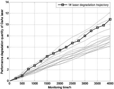
Fig. 4Comparison of degradation state

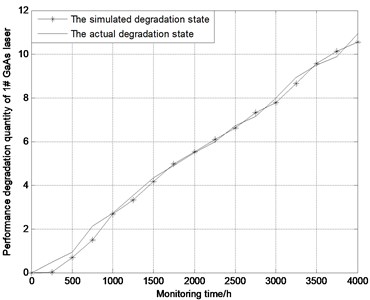
In order to quantify the degradation state comparison results, the mean square error (MSE) between the simulated degradation state and the actual observed degradation state is calculated by:

35

M S E = \frac{1}{m} \sum_{k = 1}^{m} {(\frac{y_{k} - {\hat{x}}_{k | k}}{y_{k}})}^{2},

where $m$ denotes the number of monitoring points. The MSE is only 0.066 to demonstrate fully that the parallel simulation method can simulate the laser degradation process effectively. Correspondingly, with the dynamic injection of laser performance degradation data, the parallel simulation system uses the KF algorithm and EM algorithm to execute the online evolution of $θ$ . The online parameter evolution results are shown in Fig. 5.

Fig. 5Online evolution of unknown parameters for WSSM

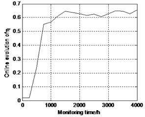
a) Online evolution results of $η$

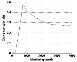
b) Online evolution results of $σ$

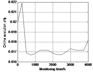
c) Online evolution results of $ϕ$

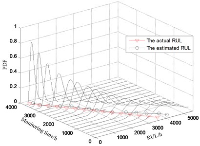
It can be easily seen that the model parameters can converge rapidly with the accumulation of observed degradation data. Fig. 5 shows that the estimated results for each parameter continually approximate the true parameter value as the available degradation data increases. The true values of $η$ , $σ$ and $ϕ$ are near 0.62, 0.27 and 0.017 respectively. The main reason for this is that the estimated results for each parameter can be real-time updated based on the newly observed degradation data as a result of the WSSM evolution mechanism. Furthermore, it shows that the KF-EM algorithm has good performance on the convergence speed in that the parameters evolution of each iteration for the KF-EM algorithm has an analytical expression. In other words, each iteration of KF-EM algorithm can be conducted with one single calculation, which results in a particularly fast and simple evolution procedure. The result reveals that the parameters evolution process of WSSM can achieve a fast convergence as the obtained degradation data increases. At each monitoring point, once the parameters in the model are evolved online, the corresponding RUL and its PDF can be calculated in real time by Eqs. (33-34). Fig. 6 shows the PDF curves predicted at 15 different monitoring time points from 250 h to 3750 h.

As shown in Fig. 6, the actual RUL falls within the range of the estimated PDF of the RUL at each monitoring point and the prognostic RUL approximates the actual RUL. Further, the estimated PDF of the RUL becomes sharper and narrower as the laser performance degradation data is accumulated. This implies that the WSSM parameters are more and more accurate, and the uncertainty of the estimated RUL is reduced. To sum up, the online, real-time and self-adaptive RUL prognosis of the GaAs laser is realized to support maintenance decision-making, and then the risk of equipment failure is reduced, and also the efficiency of maintenance support is improved.

Fig. 6PDF of RUL at different time point

6.3. Comparative study

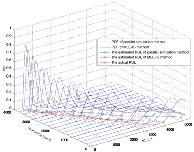
The MLE-IG method is used to estimate the drift coefficient and the diffusion coefficient offline by utilizing the degradation data of 2#-15# GaAs laser and gives $\hat{η} =$ 0.4968 and $\hat{σ} =$ 0.1941. Fig. 7 compares the estimated RUL distributions from the offline MLE-IG method with the parallel simulation method at different monitoring time points. The results show that the actual RULs of two methods fall within the range of the estimated RUL distributions at each monitoring point. However, it is observed from Fig. 7 that the PDFs of the estimated RULs for the offline MLE-IG method are typically more dispersed to reflect a stronger uncertainty. Note that the offline MLE-IG method uses the historical data to estimate the drift coefficient and diffusion coefficient and once the estimation is completed, the parameters change no longer. This results in that the effects of individual differences cannot be considered, and the model parameters cannot be evolved by utilizing the real-time monitoring data. The parallel simulation method not only overcomes the effects of Markov property and considers the influence of monitoring noise and drives the WSSM evolution driven by the real-time degradation data. As a result, the comparative results show that the parallel simulation method can effectively reduce the uncertainty of RUL prediction and improve the accuracy of RUL prediction. This further demonstrates that the proposed parallel simulation approach can estimate the RUL with lesser uncertainty and higher accuracy.

The mathematical expectation of RUL for the offline MLE-IG method at time $k$ is $E (T_{k}) = (w - y_{k}) / \hat{η}$ . From the qualitative aspect, the predicted RUL of offline MLE-IG method is much higher than the actual RUL because the latest degradation data cannot be utilized to evolve model parameters. This means that the lacking maintenance will occur and it will easily lead to an equipment breakdown, resulting in unnecessary costs or even major accidents. On the contrary, the difference between the prognostic RUL of the parallel simulation method and the actual RUL is quite little owing to the WSSM evolution.

In order to further quantify the comparison results, a loss function is employed to enable a direct comparison of the distributions for the RUL estimation between two methods. The loss function is the mean square error (MSE) about the actual RUL obtained at each monitoring point, defined as:

36

M S E_{k} = E [(T_{k} - {\tilde{T}}_{k})^{2}] = \int_{0}^{\infty} (T_{k} - {\tilde{T}}_{k})^{2} f (T_{k}| θ, Y_{k}) d T_{k},

where ${\tilde{T}}_{k}$ is the actual RUL obtained at time $k$ and $f (T_{k}| θ, Y_{k})$ is the estimated PDF of the RUL. Furthermore, the total mean square error (TMSE) is defined as the sum of MSE for all monitoring points, i.e.:

37

T M S E = \sum_{k = 1}^{m} E [(T_{k} - {\tilde{T}}_{k})^{2}] = \sum_{k = 1}^{m} \int_{0}^{\infty} (T_{k} - {\tilde{T}}_{k})^{2} f (T_{k}| θ, Y_{k}) d T_{k} .

Evidently, the smaller TMSE represents the more accurate prediction results of the RUL. The TMSE of the MLE-IG method and the parallel simulation method at different monitoring time points are 1.3399×10⁹ and 1.4004×10⁸ respectively. The results show that the accuracy of RUL prediction based on the parallel simulation is much higher than that of the MLE-IG method, implying the effectiveness of the parallel simulation method.

Fig. 7Comparison between two methods

7. Conclusions

Aiming at the problem of adaptive prediction for equipment RUL, the parallel simulation technology is introduced into the field of equipment maintenance support and the framework of parallel simulation based adaptive prediction for equipment RUL is proposed which is validated by the degradation data of GaAs laser. The case study results show that the parallel simulation method can evolve the simulation model by utilizing the real-time degradation data, i.e., the model parameters are updated, and the model output is corrected. As a result, the prognostic accuracy is improved, and the online, real-time and adaptive RUL predictions are realized. The further study includes:

1) Parallel simulation based adaptive RUL prediction for nonlinear degradation equipment. The parallel simulation method in this paper is suitable for simulating the linear performance degradation process of equipment, and the prediction accuracy will be reduced obviously when the degradation process is strong nonlinear. So, the parallel simulation based adaptive RUL prediction for nonlinear degradation equipment should be studied.

2) Model adaptive selection technology for parallel simulation. Due to the effects of the complex environmental factors, the performance degradation process has a strong uncertainty which presents the characteristic of multi-stage degradation. As a result, it is required to select the appropriate simulation model adaptively by using the real-time degradation data.

References

Wang W. B., Carr M., Xu W. J., et al. A model for residual life prediction based on Brownian motion with an adaptive drift. Microelectronics Reliability, Vol. 51, 2011, p. 285-293.

Publisher
Camci F., Chinnam R. B. Health state estimation and prognostics in machining processes. IEEE Transactions on Automation Science and Engineering, Vol. 7, Issue 3, 2010, p. 581-597.

Publisher
Gebraeel N., Elwany A., Pan J. Residual life predictions in the absence of prior degradation knowledge. IEEE Transactions on Reliability, Vol. 58, Issue 1, 2009, p. 106-117.

Publisher
Lu C. J., Meeker W. Q. Using degradation measures to estimate a time-to-failure distribution. Technometrics, Vol. 35, Issue 2, 1993, p. 161-174.

Publisher
Zhou Z. J., Hu C. H. An effective hybrid approach based on grey and ARMA for forecasting gyro drift. Chaos, Solitons and Fractals, Vol. 35, Issue 3, 2008, p. 525-529.

Publisher
Gebraeel N. Z., Lawley M. A., Liu R., et al. Residual life predictions from vibration-based degradation signals: a neural network approach. IEEE Transactions on Industrial Electronics, Vol. 51, Issue 3, 2004, p. 694-700.

Publisher
You M. Y., Meng G. A generalized similarity measure for similarity-based residual life prediction. Journal of Process Mechanical Engineering, Vol. 225, Issue 3, 2011, p. 151-160.

Publisher
Soualhi A., Razik H., Clerc G., et al. Prognosis of bearing failures using hidden Markov models and the adaptive Neuro-fuzzy inference system. IEEE Transactions on Industrial Electronics, Vol. 61, Issue 6, 2014, p. 2864-2874.

Publisher
Loutas T. H., Roulias D., Georgoulas G. Remaining useful life estimation in rolling bearing utilizing data-driven probabilistic e-support vectors regression. IEEE Transactions on Reliability, Vol. 62, Issue 4, 2013, p. 821-862.

Publisher
Carr M., Wang W. B. An approximate algorithm for prognostic modeling using condition monitoring information. European Journal of Operational Research, Vol. 211, Issue 1, 2011, p. 90-96.

Publisher
Khorasgani H., Biswas G., Sankararaman S. Methodologies for system-level remaining useful life prediction. Reliability Engineering and System Safety, Vol. 151, Issue 1, 2016, p. 8-18.

Publisher
Li X., Lv C., Wang Z. L., et al. Self-adaptive health condition prediction considering dynamic transfer of degradation mode. Acta Automatica Sinica, Vol. 40, Issue 9, 2014, p. 1889-1895.

Search CrossRef
Doksum K. A., Hoyland A. Models for variable-stress accelerated life testing experiments based on Wiener processes and the inverse Gaussian distribution. Technometrics, Vol. 34, Issue 1, 1992, p. 74-82.

Publisher
Whitmore G., Schenkelberg F. Modelling accelerated degradation data using Wiener diffusion with a time scale transformation. Lifetime Data Analysis, Vol. 3, Issue 1, 1997, p. 27-45.

Publisher
Si X. S., Wang W. B., Hu C. H., et al. Remaining useful life estimation based on a nonlinear diffusion degradation process. IEEE Transactions on Reliability, Vol. 61, Issue 1, 2012, p. 50-67.

Publisher
Whitmore G. Estimating degradation by a Wiener diffusion process subject to measurement error. Lifetime Data Analysis, Vol. 1, Issue 3, 1995, p. 307-319.

Publisher
Peng C., Teseng S. Mis-specification analysis of linear degradation models. IEEE Transactions on Reliability, Vol. 58, Issue 3, 2009, p. 444-455.

Publisher
Si X. S., Wang W. B., Hu C. H., et al. A Wiener-process-based degradation model with a recursive filter algorithm for remaining useful life estimation. Mechanical Systems and Signal Processing, Vol. 35, Issues 1-2, 2011, p. 219-237.

Publisher
Ge C. L., Zhu Y. C., Di Y. Q., et al. Basic theoretical issues of equipment parallel simulation technology. System Engineering and Electronics, Vol. 39, Issue 5, 2017, p. 1169-1177, (in Chinese).

Search CrossRef
Wang F. Y. Parallel control and management for intelligent transportation systems: concepts, architectures, and applications. IEEE Transactions on Intelligent Transportation Systems, Vol. 11, Issue 3, 2010, p. 630-638.

Publisher
Chen B. KD-ACP: a software framework for social computing in emergency management. Mathematical Problems in Engineering, Vol. 21, Issue 3, 2014, p. 35-38.

Search CrossRef
Jin H., Jespersen D., Mehrotra P., et al. High performance computing using MPI and OpenMP on multi-core parallel systems. Parallel Computing, Vol. 37, Issue 9, 2011, p. 562-575.

Publisher
Lin J. N., Jiang J., Sun L. Y., et al. Research of resource selection algorithm of parallel simulation system for command decisions support driven by real-time intelligence. Theory, Methodology, Tools and Applications for Modeling and Simulation of Complex Systems, Vol. 643, 2016, p. 419-430.

Publisher
Ge C. L., Zhu Y. C., Di Y. Q., et al. Equipment residual useful life prediction oriented parallel simulation framework. Theory, Methodology, Tools and Applications for Modeling and Simulation of Complex Systems, Vol. 643, 2016, p. 377-386.

Publisher
Si X. S., Wang W. B., Hu C. H., et al. Remaining useful life estimation – a review on the statistical data driven approaches. European Journal of Operational Research, Vol. 213, Issue 1, 2011, p. 1-14.

Publisher
Kalman R. E. A new approach to linear filtering and prediction problems. Journal of Basic Engineering, Vol. 82, 1960, p. 35-45.

Publisher
Si X. S., Wang W. B., Chen M. Y., et al. A degradation path-dependent approach for remaining useful life estimation with an exact and closed-form solution. European Journal of Operational Research, Vol. 226, Issue 1, 2011, p. 53-66.

Publisher
Pan D. H., Liu J. B., Cao J. D. Remaining useful life estimation using an inverse Gaussian degradation model. Neurocomputing, Vol. 185, 2016, p. 64-72.

Publisher

Cited by

Hybrid Degradation Equipment Remaining Useful Life Prediction Oriented Parallel Simulation considering Model Soft Switch

Chenglong Ge | Yuanchang Zhu | Yanqiang Di

(2019)

About this article

Received

15 August 2017

Accepted

22 January 2018

Published

15 August 2018

SUBJECTS

Fault diagnosis based on vibration signal analysis

DOI

https://doi.org/10.21595/jve.2018.18973

Keywords

parallel simulation

model evolution

remaining useful life

Kalman filter

expectation maximum

This is an open access article distributed under the Creative Commons Attribution License, which permits unrestricted use, distribution, and reproduction in any medium, provided the original work is properly cited.

Previous article in issue Previous Next article in issue Next

Research article

2021 12 02

A remaining useful life prediction method for engineering components based on intelligent product limit estimator

Xiaosheng Zeng, Pian Hu, Xiang Yu, Taotao Zhou, Jiangyuan Liu

Research article

2019 11 28

PCA based health indicator for remaining useful life prediction of wind turbine gearbox

Hemanth Mithun Praveen, Divya Shah, Krishna Dutt Pandey, Vamsi I, Sabareesh G R

Research article

2018 06 30

Remaining useful life prediction of the ball screw system based on weighted Mahalanobis distance and an exponential model

Juan Wen, Hongli Gao

Research article

2017 05 15

Application of EMD-WVD and particle filter for gearbox fault feature extraction and remaining useful life prediction

Xin Liu, Yunxian Jia, Zewen He, Jie Zhou

C. Ge, Y. Zhu, Y. Di, and Z. Dong, “Parallel simulation based adaptive prediction for equipment remaining useful life,” Journal of Vibroengineering, Vol. 20, No. 5, pp. 2027–2044, Aug. 2018, https://doi.org/10.21595/jve.2018.18973

Copy Extrica

Copied to clipboard!

TY  - JOUR
DO  - 10.21595/jve.2018.18973
UR  - https://doi.org/10.21595/jve.2018.18973
TI  - Parallel simulation based adaptive prediction for equipment remaining useful life
T2  - Journal of Vibroengineering
AU  - Ge, Chenglong
AU  - Zhu, Yuanchang
AU  - Di, Yanqiang
AU  - Dong, Zhihua
PY  - 2018
DA  - 2018/08/15
PB  - JVE International Ltd.
SP  - 2027-2044
IS  - 5
VL  - 20
SN  - 1392-8716
SN  - 2538-8460
ER  - 

Copy Ris

Copied to clipboard!

@article{Ge_2018,
	doi = {10.21595/jve.2018.18973},
	url = {https://doi.org/10.21595/jve.2018.18973},
	year = 2018,
	month = {aug},
	publisher = {{JVE} International Ltd.},
	volume = {20},
	number = {5},
	pages = {2027--2044},
	author = {Chenglong Ge and Yuanchang Zhu and Yanqiang Di and Zhihua Dong},
	title = {Parallel simulation based adaptive prediction for equipment remaining useful life},
	journal = {Journal of Vibroengineering}
}

Copy Bibtex

Copied to clipboard!

[1]C. Ge, Y. Zhu, Y. Di, and Z. Dong, “Parallel simulation based adaptive prediction for equipment remaining useful life,” Journal of Vibroengineering, vol. 20, no. 5, pp. 2027–2044, Aug. 2018, doi: 10.21595/jve.2018.18973.

Copy IEEE

Copied to clipboard!

Ge, Chenglong, Yuanchang Zhu, Yanqiang Di, and Zhihua Dong. “Parallel Simulation Based Adaptive Prediction for Equipment Remaining Useful Life.” Journal of Vibroengineering 20, no. 5 (August 15, 2018): 2027–44. https://doi.org/10.21595/jve.2018.18973.

Copy Chicago

Copied to clipboard!

Parallel simulation based adaptive prediction for equipment remaining useful life

Abstract

1. Introduction

2. Equipment parallel simulation paradigm

2.1. Concepts and characteristics

2.2. Weapon equipment and parallel simulation system

3. Evolutionary modeling framework for parallel simulation

3.1. Evolutionary modeling analysis

3.2. Framework of parallel simulation based adaptive prediction for equipment RUL

3.3. Equipment performance degradation modeling based on WSSM

3.3.1. Wiener process and offline MLE-IG method

3.3.2. WSSM

4. WSSM evolution

4.1. Kalman filter based WSSM output updating

4.2. EM algorithm based WSSM parameters evolution

4.2.1. E-step

4.2.2. M-step

5. Adaptive prediction for equipment RUL

6. Case study

6.1. GaAs laser device degradation data

6.2. WSSM dynamic evolution and RUL adaptive prognostic

6.3. Comparative study

7. Conclusions

References

Cited by

About this article

Related Articles