Abstract
The ball screw system is one of the crucial components of machine tools and predicting its remaining useful life (RUL) can enhance the reliability and safety of the entire machine tool and reduce maintenance costs. Although quite a few techniques have been developed for the fault diagnosis of the ball screw system, forecasting the RUL of the ball screw system is a remaining challenge. To make up for this deficiency, we present a model-based method to predict the RUL of the ball screw system, which consists of two parts: health indicator (HI) construction and RUL prediction. First, we develop a novel HI, weighted Mahalanobis distance (WDMD). Unlike the Mahalanobis distance (MD), which is constructed by fusing original features directly, the WDMD is formed with some selected features only, and the features are weighted before integration. Second, an exponential model is developed to describe the degradation path of the ball screw system. Then, the particle filtering algorithm is employed to combine the WDMD and the degradation model for state estimation and RUL prediction. The proposed approach is verified by a dataset obtained from an experimental system designed for accelerated life tests of the ball screw system. The results show that the WDMD has a more apparent deterioration trend than the MD and the proposed exponential model performs better than both the linear model and the nonlinear model in RUL prediction.
1. Introduction
Health monitoring is an important task in condition-based maintenance (CBM), and it focuses on two aspects: diagnostics and prognostics [1-5]. The diagnostics include detecting the presence of failure and identifying the characteristics of faults, such as types, locations, and damage levels [6-8], whereas the target of prognostics is to forecast the remaining useful life (RUL) of systems in advance [9, 10]. With accurate RUL prediction results, predictive maintenance or replacement can be arranged to occur at an appropriate time, which can reduce the unnecessary costs caused by unscheduled maintenance. Therefore, RUL prediction has triggered a growing amount of research recently.
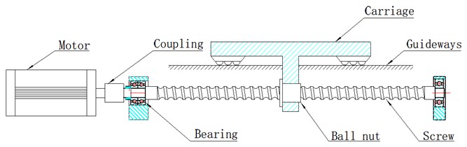
The ball screw system is a basic component in machine tools, and it is used for precision positioning. A ball screw is the main part of a ball screw system, and it is assembled to the machine base with bearings [11], as illustrated in Fig. 1. Driven by a servo motor, the ball screw can transform the rotary motion into the linear motion, and then the carriage attached to the ball screw by the ball nut can move linearly. The ball screw system is an essential part of the machine tool, and its performance has a direct influence on the machining quality and the productivity of the machine tool [12]. However, the ball screw system often works under tough conditions, and it will degrade. Therefore, it is of prime significance to estimate the health status of the ball screw system and predict its RUL, which can improve the reliability and efficiency of the machine tool and reduce maintenance costs.
Fig. 1The ball screw system
Although many techniques have been developed for the fault diagnosis of the ball screw system [13-15], RUL prediction of the ball screw system is a remaining challenge. Generally, RUL prediction approaches can be classified into two categories: data-driven techniques, and model-based techniques [16]. For data-driven approaches, the RUL estimation models are established from historical data through machine learning techniques, e.g., artificial neural network [17], support vector machine [18], and neuro-fuzzy systems [19]. These methods need no prior knowledge about the concerned system but require a large amount of historical failure data. However, it is both formidable and time-consuming to acquire adequate data for the ball screw system due to the high reliability of the ball screw. In model-based approaches, empirical models are constructed to represent the deterioration process of systems. With the condition monitoring data, the model parameters and the health state of a specific system can be updated. Based on the model, the estimated health status, and the updated parameters, the probability distribution of the RUL can be obtained. Different from data-driven techniques, model-based approaches can make use of both prior knowledge and real-time monitoring information. Therefore, they may work well in the prognostics of the ball screw system. However, some challenges still remain in the model-based methods.
One challenge of model-based prognostics is how to establish an appropriate health indicator (HI) of the plant damage level. With a proper HI, the degradation modeling can be simplified, and the prediction accuracy can be improved. Features extracted by signal processing techniques have been widely used as HIs. Camci et al. used time-domain features to reflect the bearing health state and presented a strategy to evaluate the quality of features for prognostics [20]. Kim et al. employed frequency-domain features to identify degradation states [21]. Singleton et al. obtained a bearing HI by using the Choi–Williams distribution and proved that the time-frequency-domain feature could indicate the bearing’s performance in its incipient stage of deterioration [2]. The above features depict signals from different aspects, and any given feature is only sensitive to a particular defect in a specific deterioration stage [2, 22]. During the degradation process of the ball screw system, various faults may co-occur, and thus the health state of the ball screw system cannot be represented with one feature or several features extracted from one domain. To obtain a suitable HI, we should take advantage of multiple features in different domains. Nie et al. presented an HI construction approach which utilized the Mahalanobis distance (MD) to fuse various features [23]. Then, Wang et al. applied this strategy to bearing prognostics [24]. Using the MD, the information buried in multiple features can be integrated into a single index. However, some features may have a weak correlation with the degradation process and will have no effect or even negative influence on the incorporation result. Therefore, in this paper, the original features extracted with different signal processing techniques are evaluated, and the representative ones are selected and weighted to form a novel HI named weighted Mahalanobis distance (WDMD).
Another challenge of the model-based approach is building a suitable model to describe the equipment degradation process. Peng and Tseng proposed a general linear model to predict the mean-time-to-failure of products [25]. Liu et al. developed a nonlinear autoregressive model to depict the nonlinear degradation process and used particle filtering (PF) to combine the model and condition monitoring data for RUL prediction. Zhao et al. utilized the Paris model to describe the propagation of the gear crack and forecast the failure time distribution with Bayesian inference [26]. Gebraeel et al. presented an exponential model to represent the deterioration process of bearings [27]. Si presented a nonlinear model based prognostics method and applied it to battery RUL prediction [28]. Among these studies, the exponential model is one of the most prevalent models. Since the exponential model describes the exponential form degradation process well, it has been widely used for RUL prediction and has been further improved by many investigators [9, 29-31]. Motivated by the above researches, we introduce an exponential model for the degradation modeling of the ball screw system. Then, the PF is employed to integrate the real-time HI with the degradation model for state estimation and RUL prediction.
The major contributions of this work are summarized as following:
1) A model-based approach is introduced for ball screw system RUL prediction, which is a novel attempt in machine CBM.
2) A new HI, i.e., WDMD, is proposed, which is an improvement of the MD presented in [23]. Unlike the MD, the WDMD is formed from selected features only, and they are weighted before integration. Hence, the WDMD can be more sensitive to the defect development of the ball screw system.
3) Based on the previous studies in degradation modeling, a new exponential model is presented to describe the deterioration path of the ball screw system.
The rest of this paper is organized as follows. Section 2 introduces the basic theory about the PF. The proposed model-based method for RUL prediction of the ball screw system is described in Section 3, and Section 4 implements the proposed approach with a dataset acquired from an experimental system designed for accelerated tests of the ball screw system. The study’s conclusions are presented in Section 5.
2. Particle filtering
The PF is an algorithm which attempts to approximate the system state by a series of particles with corresponding weights. Unlike the Kalman filtering, the PF is not restricted to the Gaussian assumption, and it can also address nonlinear problems. Accordingly, the PF has been widely used for prognostics [31-33].
2.1. Bayesian theory
Most dynamic systems can be described by the following two models: a process model and an observation model:
where is the actual state at time , and denotes the corresponding observation. and represent the state transition function and the observation function, respectively. is the independent and identically distributed (i.i.d.) process noise, whereas is the i.i.d. observation noise.
Let and denote all the available states and observations, respectively, and suppose the states follow a first order Markov process, i.e., . With the application of the Bayesian theory, the posterior probability density function (PDF) of the state at , namely, , can be calculated recursively using the following equations:
where stands for the prior PDF at , and is the transition density determined by the process model. denotes the likelihood defined by the observation model, and represents the evidence, as expressed by:
2.2. Particle filtering
Generally, it is impractical to solve Eq. (3) and Eq. (4) analytically, so the PF is utilized to approximate the posterior PDF by:
where represents the particles, and denotes the associated weights. is the number of particles, and stands for the Dirac function.
Particles are sampled from an importance PDF , and their weights can be calculated by:
For easy implementation, the transition density, , is often selected as the importance PDF, i.e., , and then Eq. (7) becomes:
The procedures of the standard PF are summarized as following [34]:
1) Initialization: Set 0, and sample particles from the initial distribution . Also, initialize the weight of each particle as .
2) Importance sampling: Set 1, and calculate the transition density with Eq. (1). Set the importance PDF , and then draw particles from it.
3) Weights updating: Update the weights with newly obtained measurements with Eq. (7), and then normalize the weights with the following:
4) Resampling: Remove particles with small weights and copy particles with large weights. A resampling implementation is described in detail as following [33]:
a) Set 1: , and generate a random value from the uniform distribution .
b) Set 1: , and calculate the cumulative distribution function of weights as . If , duplicate as a new particle with the weight of , and go back to Step a; otherwise, set , and return to Step b.
5) State estimation: Estimate the current state with the resampled particles and the associated weights by:
Then, return to Step 2 and repeat Step 2–5 for the next inspection time.
3. The framework of the proposed method
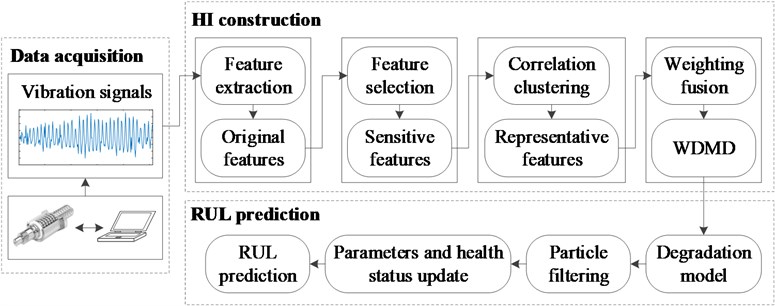
In this work, we propose a model-based method for ball screw system prognostics. Vibration data collected from an experimental system for accelerated life tests of the ball screw system are employed to validate the presented methodology. The prognostic approach consists of two modules: HI construction and RUL prediction, as shown in Fig. 2. In the first module, multiple original features are extracted from the signals with multiple signal processing techniques, and then these features are selected and weighted to form the new HI, WDMD. In the second module, the PF is utilized to integrate the proposed exponential model with the real-time WDMD for health state estimation and parameters update, and then the RUL can be predicted. More detailed information about the presented approach is provided below.
Fig. 2Flowchart of the proposed method
3.1. HI construction
3.1.1. Generation of original features
In this section, the original features are obtained with time-domain techniques, time-frequency-domain techniques, and trigonometric functions [35].
Time-domain methods often calculate signal statistics to indicate a specific system’s health state. In this investigation, ten statistics features are utilized as initial features. Time-frequency methods attempt to mine signal characteristics simultaneously from both the time domain and the frequency domain, and they are very suitable for the analysis of nonlinear and nonstationary signals. In this study, two widely used time-frequency methods, wavelet packet decomposition (WPD) and empirical mode decomposition (EMD), are used to extract the time-frequency-domain features. Specifically, the vibration data are analyzed by the WPD for three layers, and the features are produced by computing the energies and the energy ratios of coefficients in nodes. Additionally, the EMD is employed to decompose the vibration signals, and a series of components called intrinsic mode functions (IMFs) are generated. Twelve features are obtained by calculating the energy moments of the former six IMFs and their ratios according to Eq. (11) and Eq. (12), respectively [36]:
where denotes the number of the data points, and is the sequence number of a data point. represents the sampling interval of a signal, and is the th IMF.
In addition to the above features, two features are also extracted with trigonometric functions. Specifically, the raw vibration signals are first transformed to different scales using trigonometric functions, and then the standard deviations (SDs) of the scaled sequences are calculated as features [35]. In this research, two trigonometric functions, the inverse hyperbolic sine and the inverse tangent, are selected to process the vibration data, and the two corresponding features are obtained using the following two equations:
Although the presented method is based on the 40 original features shown in Table 1, it is not restricted to them. After generating enough initial features that represent the degradation of the ball screw system from multiple perspectives, we attempt to mine the most useful information hidden in these features to form an appropriate HI for RUL prediction, which is described in detail below.
Table 1The original feature set extracted from the vibration data of the ball screw system
Class | Feature | |
Time-domain features | Y1: Average absolute amplitude | Y2: Skewness |
Y3: Kurtosis | Y4: Root mean square | |
Y5: Waveform factor | Y6: Crest factor | |
Y7: Impact factor | Y8: Peak-to-peak value | |
Y9: Standard deviation | Y10: Clearance factor | |
Time-frequency-domain features | Y11-Y18: Energies of eight wavelet packet coefficients | |
Y19-Y26: Energy ratios of eight wavelet packet coefficients | ||
Y27-Y32: Energy moments of the former six IMFs | ||
Y33-Y38: Energy moment ratios of the former six IMFs | ||
Features extracted with trigonometric functions | Y39: SD of asinh(X) | |
Y40: SD of atan(X) | ||
3.1.2. Feature selection
To accurately represent the performance of the ball screw system, a group of original features are generated from the signals, as described in Section 3.1.1. However, some features are not sensitive to the damage propagation, which may have a negative effect on the HI construction. Consequently, we need to select the most effective features to construct the HI. In this paper, a widely used index, trendability, is employed to measure the quality of features. The trendability is defined by Eq. (15), and it reflects the correlation between a feature and the time [37]:
where denotes the inspection time instants during the working life of the ball screw system, is the th original feature illustrated in Table 1, and represents the total number of time indexes. and stand for the average values of and , respectively. The results obtained by Eq. (15) are confined in the range [0, 1]. A feature with a higher trendability correlates more to the degradation process, and it is more proper for RUL prediction.
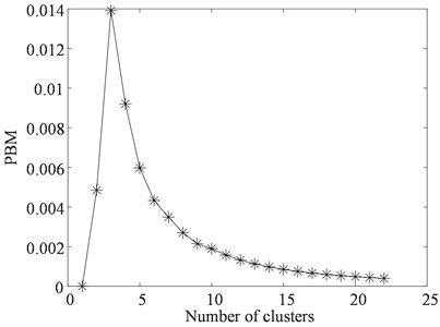
To remove features which are not obviously relevant to the deterioration development of the ball screw system, only the features whose trendability values exceed 0.5 are chosen for further processing. However, some of the selected features may represent similar variation trends, and they may have the same influence on the HI construction. To reduce the computational cost, the redundant information needs to be identified and removed. In this study, a correlation clustering algorithm [38] is used to recognize the similar features according to their correlations between each other. To determine the number of clusters, a PBM-index [39] is introduced, which is described by:
where denotes the number of the clusters, and is a given constant. Here, with , and:
is the number of features, is a partition matrix. denotes the correlation coefficient between the th clustering center and the th feature. represents the correlation coefficient between the center of the th cluster and the center of the th cluster. The actual number of clusters is the that maximizes the PBM-index.
After determining the number of clusters, the selected features are divided into several classes. Let the number of clusters be , and there are classes. Features which contain similar information about the deterioration evolution are clustered into one class, and the feature with the highest trendability in each class is selected as the representative feature of its class. Accordingly, representative features are obtained after this procedure.
3.1.3. Feature fusion
In order to take advantage of multiple features and fuse the useful information they represent, the MD is employed to integrate them into an HI [23]. Specifically, the HI is formed by calculating the MD between the given feature vector and the set of feature vectors obtained in normal conditions; this reflects the deviation of the status at a certain inspection interval from the healthy state. Therefore, the MD can indicate the health state of the equipment. During this process, each feature is treated equally, and thus they make the same contribution to the fusion result. However, the features may have different sensitivities to the defect development of the ball screw system, and those with high sensitivity should have a large impact on the integration process. Hence, an HI called WDMD is developed based on the MD in this paper, as defined by:
where denotes the feature vector composed of representative features at , is the covariance matrix of a dataset that contains feature vectors consisting of typical features obtained in the healthy state, and represents the mean of the data set. Here:
where denotes the normalized weight of the representative feature , i.e., , which reflects its sensitivity to the degradation of the ball screw system.
3.2. RUL prediction
Due to the complex and heterogeneous working conditions, the ball screw system usually deteriorates stochastically. Therefore, we attempt to describe the degradation path of the ball screw system with an exponential Wiener process model, as denoted by:
where is a random variable, and is a centered Brownian motion representing the stochastic effect.
For convenience, Eq. (20) is transformed into a linear form by using the logged observations, as represented by:
According to Eq. (21), we can obtain the following difference equation:
where obeys with . For simplicity, let represent the model parameters.
After degradation modeling, the model parameters and the health state of the system can be estimated by combining the model and the condition monitoring information. At let represent the available logged measurements, and suppose the model parameters are known. Because the error increments are i.i.d. normal random variables, the conditional joint PDF of can be obtained by:
In practice, the parameters are usually unknown. However, based on their prior PDF and Eq. (23), we can determine their joint posterior PDF at through the Bayesian theory. After the health state estimation and parameters update, the PDF of the RUL at can be predicted.
The definition of the RUL at can be expressed as:
where represents the lower bound of a variable, is a predefined failure threshold, and is the predicted health state at , which can be calculated by:
According to the independent increment property of the Brownian motion, the PDF of the RUL at can be represented as:
In this paper, the PF is utilized to combine the HI and the degradation model for updating parameters, estimating the health state, and predicting the RUL. To update the parameters along with the health status, parameters and are regarded as latent states of the system as well as the health state . Then the state space model of the system become , and the RUL prediction process with the PF includes the following steps:
1) At initial time , sample particles from the initial distribution and initialize the particle weights by .
2) Once a new measurement is obtained at , sample particles according to the importance PDF defined by the following state transition functions:
3) Update the particle weights by:
4) Resample particles from according to , using the resampling algorithm described in Section 2.2.
5) Update the health state and the model parameters at with Eq. (10).
6) With the estimated HI, , and the model parameters, and , predict the RUL by:
7) Set , return to Step 2 and repeat Step 2-6 until .
4. Applications and discussions
In this section, a dataset collected from an experimental system designed for accelerated life tests of the ball screw system is utilized to validate the proposed method’s effectiveness.
4.1. Experimental system and vibration data
Since the ball screw is a highly reliable product, it usually takes a long time for the ball screw system to fail. Consequently, it is difficult to acquire the condition monitoring data during the entire working life of the ball screw system. To make up for this deficiency, we designed and manufactured an experimental system to conduct accelerated life tests for the ball screw system. With the experimental platform, the degradation speed of the ball screw system is expedited by increasing the system load, which causes the time amount for the system to become invalid to be reduced. Thus, adequate degradation data can be collected to study ball screw system diagnostics and prognostics. Fig. 3 shows the overview of the experimental system, and it consists of two parts: the testbed for the accelerated life test of the ball screw system, and the control cabinet.
The testbed depicted in Fig. 4 can simulate the actual movement of the ball screw system and exert the load on the ball screw. To collect the condition monitoring data, two uniaxial accelerometers are fixed on the bearings at the drive end and the floating end, respectively, and a triaxial accelerometer is attached to the ball nut, as illustrated in Fig. 5. The main dimensions of the ball screw are listed in Table 2. During the testing process, the rotating speed was 1,000 rpm, and the screw rotation was controlled by the servo motor. The ball screw was subjected to a load of 100 N axially throughout the test, which was produced by the magnetic powder brake and transmitted by the gear and rack.
Fig. 3The experimental system for accelerated life tests of the ball screw system
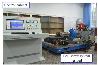
Fig. 4The testbed for accelerated life tests of the ball screw system
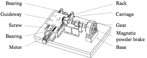
Fig. 5Installation positions of accelerometers
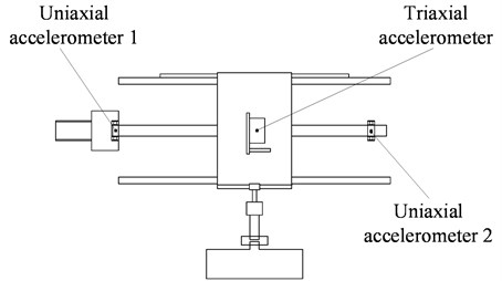
Table 2Parameters of the ball screw
Parameters | Value |
Screw diameter (mm) | 40 |
Screw length (mm) | 750 |
Screw pitch (mm) | 10 |
Ball diameter (mm) | 7.144 |
Circles of nut | 3 |
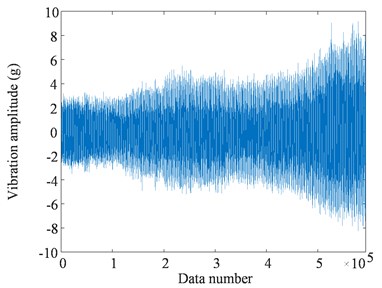
In the test, vibration signals were collected every 30 min, and the sampling frequency was 5,000 Hz. We used a digital microscope to observe the wear status of the ball screw and take pictures, as described in Fig. 6. With the microscope, we can obtain the enlarged view of the ball screw, as illustrated in Fig. 6(b). By increasing the magnification times, we can see more details about the condition of the ball screw, as shown in Fig. 6(c) and Fig. 6(d), which display the photographs of the ball groove before and after the test, respectively. It is seen that pittings appeared on the surface of the screw at the end of the test. Vibration signals acquired from uniaxial accelerometer 1 throughout the test are shown in Fig. 7. In the beginning, the vibration data remained relatively stable, and then small increases occurred. In the late stage of the degradation, the signals increased rapidly until the ball screw system failed.
Fig. 6a) The screw, b) the enlarged view of the screw, c) the enlarged view of the ball groove before the test, d) the enlarged view of the ball groove after the test
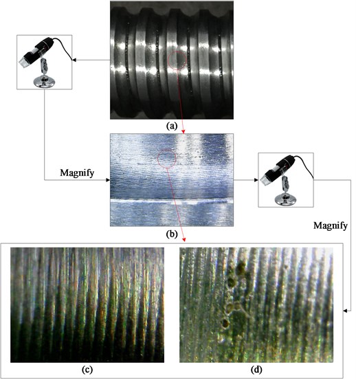
Fig. 7Vibration signals of the ball screw system
4.2. HI construction of the ball screw system
To construct the HI for the ball screw system, 40 original features, as listed in Table 1, were extracted from the raw vibration data. Then we calculated the trendability of each feature, as depicted in Fig. 8. To select features that appropriately correlated to the defect development and propagation, features whose values of trendability were 0.5 or below were removed, and then 22 features were obtained. To identify the redundant information among these features, they were clustered with the correlation clustering algorithm; the PBM-index values with different cluster numbers are shown in Fig. 9. The index achieved its maximum value when 3, so these 22 features were divided into three classes. After clustering, the feature with the highest trendability in each class was chosen as the representative feature for its cluster. Accordingly, we obtained three typical features for feature fusion. To compare the representative features, they were normalized and displayed in Fig. 10. It is observed that different typical features represent distinct deterioration trends of the ball screw system. Specifically, Y5 contains abundant information about the early stage of the degradation, and Y12 describes the fluctuation in the middle of the damage propagation. Furthermore, Y32 is sensitive to the late stage of the degradation.
Fig. 8Trendability of original features
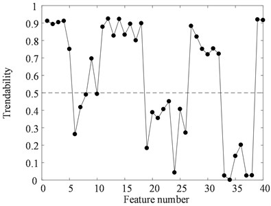
Fig. 9PBM-index values with different cluster numbers
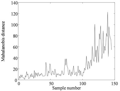
To take advantage of each typical feature, the MD was employed to fuse the information represented by the features. Before calculating the MD, the representative features were weighted according to their values of trendability. Then we could obtain the WDMD at any measurement time using Eq. (18), as depicted in Fig. 11. To verify the benefits of the WDMD, the MD of 40 original features were calculated for comparison, as shown in Fig. 12. It is seen that the WDMD indicates a more evident deterioration tendency during the entire lifecycle. To compare these two HIs quantitatively, the trendability values of the WDMD and the MD were calculated, as illustrated in Table 3, and it is found that the trendability value of the WDMD is higher than that of the MD. Therefore, the WDMD is more sensitive to the degradation development of the ball screw system, and it is more suitable for RUL prediction.
Fig. 10Representative features
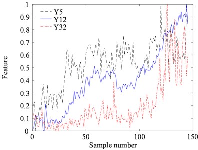
Fig. 11The WDMD of the ball screw system
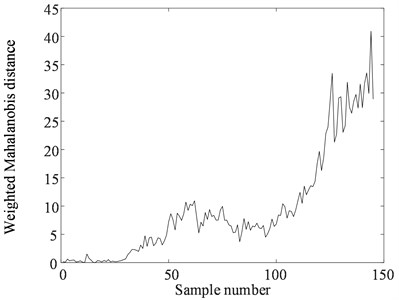
Table 3Trendability values of the WDMD and the MD
Health indicator | MD | WDMD |
Trendability | 0.6013 | 0.8525 |
Fig. 12The MD of the ball screw system
4.3. RUL prediction of the ball screw system
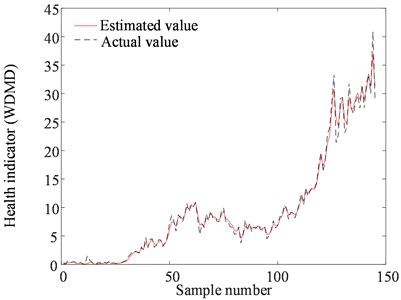
In this section, the PF was used to integrate the WDMD with the presented exponential model for model parameters update, health state estimation, and RUL prediction. The number of particles was set to be 1,000. Fig. 13 shows the estimation results of the WDMD during the whole degradation process, and it is seen that the proposed model can track the deterioration path well.
Fig. 13WDMD estimation results.
The update process of the model parameters and is displayed in Fig. 14. As more measurements became available, converged to a stable value after 12 samples with fast speed. In contrast, experienced fluctuations during the estimation process. At each inspection time index, the PDF of the RUL can be predicted with the estimated health state and model parameters.
Fig. 14The update process of model parameters: a) β, b) σ
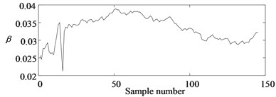
a)
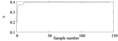
b)
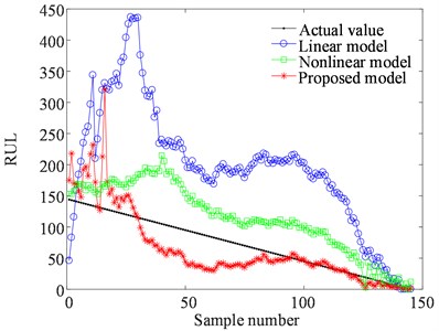
To manifest the merits of the presented model, both the linear Wiener process model [40] and the nonlinear Wiener process model [28] were employed for comparison. The means of the predicted RUL by three models at different measurement intervals are shown in Fig. 15. The proposed model converged to the real RUL after 83 points, whereas the other two models differed greatly from the actual RUL value at this stage. Among these three models, the linear model generated the largest prediction errors, because the degradation of the ball screw system did not increase linearly. The RUL estimation results of the nonlinear model were more accurate than those of the linear model, but it also could not estimate the RUL accurately until the end of the deterioration stage. For the presented exponential model, it forecasted the RUL with large errors in the beginning since there were not enough WDMD values. As more measurements became available, the prediction errors were reduced, and the predicted value converged to the real RUL gradually.
Fig. 15The means of the predicted RUL by three models at different inspection time indexes
To compare the models mentioned above quantitatively, we calculated the prediction errors at by:
where is the real value of the RUL, and denotes the predicted RUL.
The prediction errors of the three models at all time indexes were calculated using Eq. (30). For comparison, we divided the results of each model into three intervals and calculated the percentage of points in each interval, as shown in Table 4. It is observed that the proposed model predicts the RUL for 52.08 % of points with a prediction error of no higher than 30 %, whereas the nonlinear model’s percentage of points with prediction errors of 50 % or lower is only 30.56 %. The linear model estimates only 4.86 % of points with prediction errors of 50 % or lower. Therefore, the proposed model can predict the RUL of the ball screw system with the lowest prediction error.
Table 4Comparison of prediction errors produced by different models
Model | The percentage of points lying in different prediction error intervals | ||
30 % | 30 % 50 % | 50 % | |
Linear model | 2.08 % | 2.78 % | 95.14 % |
Nonlinear model | 13.19 % | 17.36 % | 69.44 % |
Proposed model | 52.08 % | 27.78 % | 20.14 % |
The superior properties of the presented model can be explained as follows. The ball screw system deterioration has an exponentially growing trend comprehensively, so that the exponential model can describe the degradation process best. In addition, the Brownian motion parameter is considered and updated with the PF in our method, which can indicate the Brownian error in real time. Hence, the proposed model can improve the accuracy of ball screw system RUL estimation.
5. Conclusions
In this study, we introduced a model-based method for ball screw system RUL prediction. First, we developed a new HI, named WDMD, by weighted fusion of selected features, and the experimental results show that the WDMD is more sensitive to the degradation process of the ball screw system than the MD and is therefore more suitable for ball screw system RUL prediction. Second, we introduced an exponential Wiener process model to describe the degradation path of the ball screw system. Compared with the linear model and the nonlinear model, the exponential model generates the best RUL prediction results.
However, there are still some restrictions in this study. For instance, the proposed method cannot estimate the RUL accurately during the first half of the ball screw system’s lifetime because of fluctuations. At these time indexes, the exponential model is not capable of describing the deterioration, and then the corresponding predicted RUL has a large gap with the actual value. Consequently, future work will consider developing more general models to comprehensively enhance the RUL prediction accuracy of the ball screw system.
References
-
Jardine A. K. S., Lin D., Banjevic D. A review on machinery diagnostics and prognostics implementing condition-based maintenance. Mechanical Systems and Signal Processing, Vol. 20, Issue 7, 2006, p. 1483-1510.
-
Singleton R. K., Strangas E. G., Aviyente S. Extended Kalman filtering for remaining-useful-life estimation of bearings. IEEE Transactions on Industrial Electronics, Vol. 62, Issue 3, 2015, p. 1781-1790.
-
Feng Z., Zuo M. J. Vibration signal models for fault diagnosis of planetary gearboxes. Journal of Sound and Vibration, Vol. 331, Issue 22, 2012, p. 4919-4939.
-
Mao W., He L., Yan Y., Wang J. Online sequential prediction of bearings imbalanced fault diagnosis by extreme learning machine. Mechanical Systems and Signal Processing, Vol. 83, 2017, p. 450-473.
-
Liang X., Zuo M. J., Feng Z. Dynamic modeling of gearbox faults: a review. Mechanical Systems and Signal Processing, Vol. 98, 2018, p. 852-876.
-
Li Y., Xu M., Wang R., Huang W. A fault diagnosis scheme for rolling bearing based on local mean decomposition and improved multiscale fuzzy entropy. Journal of Sound and Vibration, Vol. 360, 2016, p. 277-299.
-
Guo L., Gao H., Huang H., He X., Li S. C. Multifeatures fusion and nonlinear dimension reduction for intelligent bearing condition monitoring. Shock and Vibration, Vol. 2016, 2016, p. 4632562.
-
Lei Y., Zuo M. J. Gear crack level identification based on weighted K nearest neighbor classification algorithm. Mechanical Systems and Signal Processing, Vol. 23, Issue 5, 2009, p. 1535-1547.
-
Guo L., Li N., Jia F., Lei Y., Lin J. A recurrent neural network based health indicator for remaining useful life prediction of bearings. Neurocomputing, Vol. 240, 2017, p. 98-109.
-
Si X.-S., Wang W., Chen M.-Y., Hu C.-H., Zhou D.-H. A degradation path-dependent approach for remaining useful life estimation with an exact and closed-form solution. European Journal of Operational Research, Vol. 226, Issue 1, 2013, p. 53-66.
-
Vicente D. A., Hecker R. L., Villegas F. J., Flores G. M. Modeling and vibration mode analysis of a ball screw drive. The International Journal of Advanced Manufacturing Technology, Vol. 58, Issue 1, 2012, p. 257-265.
-
Möhring H. C., Bertram O. Integrated autonomous monitoring of ball screw drives. CIRP Annals – Manufacturing Technology, Vol. 61, Issue 61, 2012, p. 355-358.
-
Tsai P. C., Cheng C. C., Hwang Y. C. Ball screw preload loss detection using ball pass frequency. Mechanical Systems and Signal Processing, Vol. 48, Issues 1-2, 2014, p. 77-91.
-
Jin W. A comparative study of fault detection and health assessment techniques for motion control mechanism. Chemical Engineer, Vol. 140, Issue 8, 2014, p. 473-482.
-
Feng G. H., Pan Y. L. Establishing a cost-effective sensing system and signal processing method to diagnose preload levels of ball screws. Mechanical Systems and Signal Processing, Vol. 28, Issue 2, 2012, p. 78-88.
-
Kan M. S., Tan A. C. C., Mathew J. A review on prognostic techniques for non-stationary and non-linear rotating systems. Mechanical Systems and Signal Processing, Vol. 62, Issue 63, 2015, p. 1-20.
-
Tian Z., Wong L., Safaei N. A neural network approach for remaining useful life prediction utilizing both failure and suspension histories. Mechanical Systems and Signal Processing, Vol. 24, Issue 5, 2010, p. 1542-1555.
-
Tran V. T., Hong T. P., Yang B. S., Tan T. N. Machine performance degradation assessment and remaining useful life prediction using proportional hazard model and support vector machine. Mechanical Systems and Signal Processing, Vol. 32, Issue 4, 2012, p. 320-330.
-
Chen C., Vachtsevanos G., Orchard M. E. Machine remaining useful life prediction: an integrated adaptive neuro-fuzzy and high-order particle filtering approach. Mechanical Systems and Signal Processing, Vol. 28, Issue 9, 2012, p. 597-607.
-
Camci F., Medjaher K., Zerhouni N., Nectoux P. Feature evaluation for effective bearing prognostics. Quality and Reliability Engineering International, Vol. 29, Issue 4, 2013, p. 477-486.
-
Kim H. E., Tan A. C. C., Mathew J., Choi B. K. Bearing fault prognosis based on health state probability estimation. Expert Systems with Applications, Vol. 39, Issue 5, 2012, p. 5200-5213.
-
Qiu H., Lee J., Lin J., Yu G. Robust performance degradation assessment methods for enhanced rolling element bearing prognostics. Advanced Engineering Informatics, Vol. 17, Issues 3-4, 2003, p. 127-140.
-
Nie L., Azarian M. H., Keimasi M., Pecht M. Prognostics of ceramic capacitor temperature‐humidity‐bias reliability using Mahalanobis distance analysis. Circuit World, Vol. 33, Issue 3, 2007, p. 21-28.
-
Wang Y., Peng Y., Zi Y., Jin X., Tsui K.-L. A Two-Stage Data-Driven-Based Prognostic Approach for Bearing Degradation Problem. IEEE Transactions on Industrial Informatics, Vol. 12, Issue 3, 2016, p. 924-932.
-
Peng C. Y., Tseng S. T. Mis-specification analysis of linear degradation models. IEEE Transactions on Reliability, Vol. 58, Issue 3, 2009, p. 444-455.
-
Zhao F., Tian Z., Zeng Y. Uncertainty quantification in gear remaining useful life prediction through an integrated prognostics method. IEEE Transactions on Reliability, Vol. 62, Issue 1, 2013, p. 146-159.
-
Gebraeel N. Z., Lawley M. A., Li R., Ryan J. K. Residual-life distributions from component degradation signals: A Bayesian approach. IIE Transactions, Vol. 37, Issue 6, 2005, p. 543-557.
-
Si X.-S. An adaptive prognostic approach via nonlinear degradation modeling: application to battery data. IEEE Transactions on Industrial Electronics, Vol. 62, Issue 8, 2015, p. 5082-5096.
-
Gebraeel N., Pan J. Prognostic degradation models for computing and updating residual life distributions in a time-varying environment. IEEE Transactions on Reliability, Vol. 57, Issue 4, 2008, p. 539-550.
-
Gebraeel N. Residual-life estimation for components with non-symmetric priors. IIE Transactions, Vol. 41, Issue 4, 2009, p. 372-387.
-
Li N. P., Lei Y. G., Lin J., Ding S. X. An improved exponential model for predicting remaining useful life of rolling element bearings. IEEE Transactions on Industrial Electronics, Vol. 62, Issue 12, 2015, p. 7762-7773.
-
Orchard M. E., Vachtsevanos G. J. A particle filtering approach for on-line failure prognosis in a planetary carrier plate. International Journal of Fuzzy Logic and Intelligent Systems, Vol. 7, Issue 4, 2007, p. 221-227.
-
An D., Choi J.-H., Kim N. H. Prognostics 101: a tutorial for particle filter-based prognostics algorithm using Matlab. Reliability Engineering and System Safety, Vol. 115, 2013, p. 161-169.
-
Arulampalam M. S., Maskell S., Gordon N., Clapp T. A tutorial on particle filters for online nonlinear/non-Gaussian Bayesian tracking. IEEE Transactions on Signal Processing, Vol. 50, Issue 2, 2002, p. 174-188.
-
Javed K., Gouriveau R., Zerhouni N., Nectoux P. Enabling health monitoring approach based on vibration data for accurate prognostics. IEEE Transactions on Industrial Electronics, Vol. 62, Issue 1, 2015, p. 647-656.
-
Bin G. F., Gao J. J., Li X. J., Dhillon B. S. Early fault diagnosis of rotating machinery based on wavelet packets – empirical mode decomposition feature extraction and neural network. Mechanical Systems and Signal Processing, Vol. 27, 2012, p. 696-711.
-
Spearman C. The proof and measurement of association between two things. The American Journal of Psychology, Vol. 15, Issue 1, 1904, p. 72-101.
-
Lei Y. G., Li N. P., Gontarz S., Lin J., Radkowski S., Dybala J. A Model-based method for remaining useful life prediction of machinery. IEEE Transactions on Reliability, Vol. 65, Issue 3, 2016, p. 1314-1326.
-
Pakhira M. K., Bandyopadhyay S., Maulik U. Validity index for crisp and fuzzy clusters. Pattern Recognition, Vol. 37, Issue 3, 2004, p. 487-501.
-
Si X.-S., Wang W., Hu C.-H., Chen M.-Y., Zhou D.-H. A Wiener-process-based degradation model with a recursive filter algorithm for remaining useful life estimation. Mechanical Systems and Signal Processing, Vol. 35, Issues 1-2, 2013, p. 219-237.
Cited by
About this article

This research was financially supported by the National Natural Science Foundation of China (Grant No. 51775452).
