Sensitivity of beam-column element stiffness matrix to the crack parameters

1. Introduction

Crack modeling and identifying constitute the important aspects in damage detection studies. A crack is defined by its location, effective length and depth, named crack parameters. Each one of the crack parameters directly affects the stiffness components. In general, a crack is modeled through FEM [1-3], stiffness reduction [4-11], and fracture mechanics [12-17] methods. Many researchers have sought and seek to find a relation between crack parameters and vibrational components like stiffness, natural frequencies and mode shapes. The Christides and Barr [6] approach, where, element stiffness around the crack is calculated in terms of distance from the center of the crack, is applied in many studies [8, 10, 11]. Sinha, et al. [7] considered linear trend for stiffness variation in the cracked region and proposed a simplified method of cracking subjects to transverse vibration by applying shape functions. Caddemi and Caliò [5] introduced an equation to the Bernoulli beam element stiffness matrix in the presence of several cracks where, the stiffness matrix is calculated based on the cracked beam vibration modes. Caddemi et al. [9] proposed a Timoshenko beam model with the rotational and translational discontinuity, which is based on modeling shear and flexural stiffness discontinuity in the form of distributed Dirac delta and Hyvsid functions. In their study, an equation is developed that provides a relation between element deformation and shape functions, which yields an explicit form of the stiffness matrix. Labib et al. [18] obtained natural frequencies by applying a rotational spring model, including partial Gaussian elimination and the Wittrick-Williams algorithm to model crack elements, where in this process, dynamic stiffness matrices of order four are obtained in a recursive manner, according to the number of cracks. The same authors [19] applied natural frequency degradations and simulated noise free and contaminated measurements in order to locate a single crack in a frame. Differences between uncracked and cracked frequencies is obtained through theoretical analysis and real measurements. Mehrjoo et al. [20] applied the Betty theory together with the ideas of conjugated beam and introduced an equation for the cracked beams regardless of the rotational moment of inertia and shear deformation. Model reduction through static condensation method is an approach applied in damage detection. Guyan and Irons are the first to propose the condensation approach for the deletion of unwanted degrees of freedom in 1965. Since late 1960s, this approach has been and is being widely applied in many static and dynamic problems, like component mode synthesis, Eigen problem analysis of large models and experimental mode expansion [21]. Static condensation is an extension of the Gauss elimination algorithm [22]. A recursive method based on static condensation to locate damage based on measured modal frequencies is applied by Ghee Koh et al. [23, 24] where a physical property adjustment model updating method is used. Implementing this method requires only a few modes measured from the damaged structure. Li et al. [25] proposed a method for locating and estimating structural damage in 2D and 3D analytical models of buildings. Damage in this context, is defined in terms of changes in element stiffness. The condensed stiffness matrix of a structure is estimated for damage detection.

In this study with the assistant of static condensation method, a new close form equation is proposed for stiffness matrix of cracked beam-column element. Sensitivity of stiffness components are studied through seven introduced dimensionless coefficients and the results are illustrated in different graphs.

2. Stiffness matrix of a cracked beam-column element

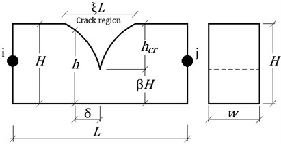
In this context, a crack is defined by its location ($\eta L$), effective length ($\xi L$) and effective depth ($h_{eff}$), which are named crack parameters. Each one of these parameters directly affects the stiffness components.

Fig. 1Cracked element and element section

2.2. Effective crack depth

By considering linear variation in stiffness changes within the above effective crack length, section height in the cracked region is calculated as follows:

3

$\frac{h}{H}=\sqrt[3]{{\beta }^3+\frac{4{\left(1-{\beta }^3\right)}^2}{3\ln \left(\frac{1}{{\beta }^3}\right)}\frac{\delta }{H}},$

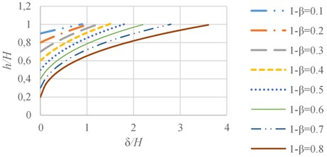
where, $\delta$ is the distance from the crack centre along its length,$\mathrm{}h$ is the section height at distance $\delta$ and $1-\beta$ is the crack to section depth ratio. Section heights within the crack region in different damage scenarios are plotted in Fig. 2. Effective crack depth ($h_{eff})$ is obtained in a manner that the area below the graph of Eq. (3) becomes equal to that of Eq. (4) within $0\le \frac{\delta }{H}\le \frac{0.75H}{1-{\beta }^3}\ln \left(\frac{1}{{\beta }^3}\right)$ limit:

4

$h_{eff}=\frac{3H}{4}\frac{{(1-\beta }^4)}{\left({1-\beta }^3\right)}.$

Fig. 2Element section height near crack, Eq. (3)

2.3. Cracked beam-column element stiffness matrix

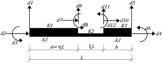
A concentrated open crack in a beam-column element is expressed by an element with twelve DOFs, Fig. 3. The crack effective length and depth are obtained through Eqs. (2)-(4), respectively. Through a model reduction approach of static condensation, crack sides’ DOFs (d7 to d12) are condensed and a new cracked element stiffness matrix is obtained. Each component of the condensed stiffness matrix is divided by its relevant component of the intact stiffness matrix which yields seven dimensionless coefficients expressed through Eq. (5), as follows:

5

$\mathrm{\varnothing }=\frac{{k_{cracked}}_{11n}}{{k_{11}}_n},{{\mathrm{\varnothing }}_1}_n=\frac{{k_{cracked}}_{11n}}{{k_{22}}_n},{{\mathrm{\varnothing }}_2}_n=\frac{{k_{cracked}}_{23n}}{{k_{23}}_n},{{\mathrm{\varnothing }}_3}_n=\frac{{k_{cracked}}_{26n}}{{k_{26}}_n},$
${{\mathrm{\varnothing }}_4}_n=\frac{{k_{cracked}}_{33n}}{{k_{33}}_n},{{\mathrm{\varnothing }}_5}_n=\frac{{k_{cracked}}_{36n}}{{k_{36}}_n},{{\mathrm{\varnothing }}_6}_n=\frac{{k_{cracked}}_{66n}}{{k_{66}}_n},$

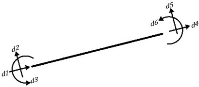
where, ${k_{cracked}}_{ijn}$ and ${k_{ij}}_n$are the cracked and intact element stiffness components, respectively. The active stiffness coefficients in different DOFs are tabulated in Table 1. The DOFs of the subject beam - column element is shown in Fig. 4.

Table 1Stiffness coefficients in different DOFs

DOF	1	2	3	4	5	6
1	$\varnothing$	0	0	$\varnothing$	0	0
2	0	${\varnothing }_1$	${\varnothing }_2$	0	${\varnothing }_1$	${\varnothing }_3$
3	0	${\varnothing }_2$	${\varnothing }_4$	0	${\varnothing }_2$	${\varnothing }_5$
4	$\varnothing$	0	0	$\varnothing$	0	0
5	0	${\varnothing }_1$	${\varnothing }_2$	0	${\varnothing }_1$	${\varnothing }_3$
6	0	${\varnothing }_3$	${\varnothing }_5$	0	${\varnothing }_3$	${\varnothing }_6$

By applying the above coefficients, stiffness matrix of the cracked elements is obtained through Eq. (6):

6

${k_{cracked}}_n=E_n{I}_n\left(\begin{array}{cccccc}{k_{11}}_n& 0& 0& {-k_{11}}_n& 0& 0\\ 0& {k_{22}}_n& {k_{23}}_n& 0& {{-k}_{22}}_n& {k_{26}}_n\\ 0& {k_{23}}_n& {k_{33}}_n& 0& {{-k}_{23}}_n& {k_{36}}_n\\ {{-k}_{11}}_n& 0& 0& {k_{11}}_n& 0& 0\\ 0& {{-k}_{22}}_n& {{-k}_{23}}_n& 0& {k_{22}}_n& {{-k}_{26}}_n\\ 0& {k_{26}}_n& {k_{36}}_n& 0& {{-k}_{26}}_n& {k_{66}}_n\end{array}\right),$
${k_{11}}_n=\frac{1}{L_n{r_n}^2}\mathrm{}\mathrm{\varnothing },\mathrm{}\mathrm{}\mathrm{}{k_{22}}_n=\frac{12}{L_n^3}{{\mathrm{\varnothing }}_1}_n,{k_{23}}_n=\frac{6}{L_n^2}{{\mathrm{\varnothing }}_2}_n,{k_{26}}_n=\frac{6}{L_n^2}{{\mathrm{\varnothing }}_3}_n,{k_{33}}_n=\frac{4}{L_n}{{\mathrm{\varnothing }}_4}_n,$
${k_{36}}_n=\frac{2}{L_n}{{\mathrm{\varnothing }}_5}_n,{k_{66}}_n=\frac{4}{L_n}{{\mathrm{\varnothing }}_6}_n,{\xi }_n=\frac{1.5h}{L\left(1-{{\beta }_n}^3\right)}\ln \left(\frac{1}{{{\beta }_n}^3}\right),$
$D={\beta }_n^6{{\xi }_n}^4-2{\beta }_n^3{{\xi }_n}^4+{{\xi }_n}^4-4{\beta }_n^6{{\xi }_n}^3+4{{\xi }_n}^3-12{\eta }_n{\beta }_n^6{{\xi }_n}^2+12{\eta }_n{{\xi }_n}^2$
$+6{\beta }_n^6{{\xi }_n}^2-6{{\xi }_n}^2-12{{\eta }_n}^2{\beta }_n^6{\xi }_n+12{{\eta }_n}^2{\xi }_n+12{\eta }_n{\beta }_n^6{\xi }_n-12{\eta }_n{\xi }_n$
$-4{\beta }_n^6{\xi }_n+4{\xi }_n+{\beta }_n^6+2{\beta }_n^3+1,$
${\mathrm{\varnothing }}_n=\frac{3\left({\beta }_n+1\right)\left({{\beta }_n}^2+1\right)}{3\left({{\beta }_n}^3+{{\beta }_n}^2+{\beta }_n+1\right)+{\xi }_n{\beta }_n+{\xi }_n{{\beta }_n}^2-3{\xi }_n{{\beta }_n}^3+{\xi }_n},$
${{\mathrm{\varnothing }}_1}_n=\frac{2{\beta }_n^3+{\beta }_n^6-\left({\beta }_n^6-1\right){\xi }_n+1}{D},$
${{\mathrm{\varnothing }}_2}_n=\frac{{\xi }_n\left(2{\eta }_n-2{\eta }_n{\beta }_n^6\right)-\left({\beta }_n^6-1\right){\xi }_n^2+2{\beta }_n^3+{\beta }_n^6+1}{D},$
${{\mathrm{\varnothing }}_3}_n=\frac{{-\xi }_n\left(2{\eta }_n-2{\eta }_n{\beta }_n^6+2{\beta }_n^6-2\right)+\left({\beta }_n^6-1\right){\xi }_n^2+2{\beta }_n^3+{\beta }_n^6+1}{D},$
${{\mathrm{\varnothing }}_4}_n=\frac{\left(3{{\eta }_n}^2-{3{{\eta }_n}^2\beta }_n^6\right){\xi }_n+\left(3{\eta }_n-{3{\eta }_n\beta }_n^6\right){{\xi }_n}^2-\left({\beta }_n^6-1\right){{\xi }_n}^3+2{\beta }_n^3+{\beta }_n^6+1}{D},$
${{\mathrm{\varnothing }}_5}_n=\frac{\left(6{{\eta }_n}^2{\beta }_n^6-6{{\eta }_n}^2-{6{\eta }_n\beta }_n^6+6{\eta }_n\right){\xi }_n-\left(6{\eta }_n-{6{\eta }_n\beta }_n^6+3{\beta }_n^6-3\right){{\xi }_n}^2}{D}$
$+\frac{\left({2\beta }_n^6-2\right){{\xi }_n}^3+2{\beta }_n^3+{\beta }_n^6+1}{D},$
${{\mathrm{\varnothing }}_6}_n=\frac{-\left(3{{\eta }_n}^2{\beta }_n^6-3{{\eta }_n}^2-{6{\eta }_n\beta }_n^6+6{\eta }_n+3{\beta }_n^6-3\right){\xi }_n+\left(3{\eta }_n-{3{\eta }_n\beta }_n^6+3{\beta }_n^6-3\right){{\xi }_n}^2}{D}$
$-\frac{\left({\beta }_n^6-1\right){{\xi }_n}^3+2{\beta }_n^3+{\beta }_n^6+1}{D},$

where, $1-{\beta }_n$ is the crack to section depth ratio, ${\eta }_n$ is the crack location from beginning of the element to element length ratio, ${\xi }_n$ is the crack effective length to element length ratio and $n$ is the element number.

Fig. 3Cracked beam column element with twelve DOFs

2.4. Assembling the global dynamic stiffness matrix

This matrix is assembled through those of the individual constituent cracked beam-columns. The stiffness matrix of each beam-column in the local coordinate system is transformed into the global coordinate system through Eq. (7) introduced by [26]:

7

${\mathbf{K}}_{Total}={\mathbf{T}}^T{\mathbf{K}}_{Local}\mathbf{T},$

where, $\mathbf{T}$ is the transformation matrix.

Fig. 4DOFs in a beam-column element

3. Numerical studies

This proposed method is verified through existing four different examples, Table 2.

3.1. Example 1

A simple cracked beam applied in Mehrjoo et al. [20] is considered here. This beam has 4 m length, 0.1 m width, and 0.2 m height. Material is of steel with Poisson’s ratio of 0.3, Table 2. The beam has a crack with 80 mm depth located 1.5 m from the left support, Fig. 5. To validate this proposed method, natural frequencies, static, and dynamic responses of this beam subjects to static and impact loads are obtained and compared to the results extracted from a simulator Abaqus, CAE 2017 software. The cracked region of the deformed beam shape at a specific time step in Abaqus software is shown in Fig. 6.

Fig. 5Simple supported beam of example 1 [20]

3.1.1. Natural frequencies

These frequencies obtained by Mehrjoo et al. [20], FEM, and these proposed methods are tabulated in Table 3, whereas observed, this proposed method is in a good agreement with its counterparts. The maximum error in this proposed method at second mode is 3.3 %.

Fig. 6Crack modelling in Abaqus

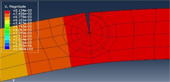
Table 3Natural frequencies obtained by Mehrjoo et al. [20], FEM, and this proposed methods

Natural frequencies of three primary modes
Mode	Mehrjoo et al. [20]	FEM (Abaqus)	Present
1	26.75	26.62	26.46
2	111.64	108.82	112.45
3	261.19	246.42	247.99

3.1.2. Static responses

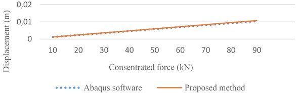
An incremental concentrated static force is exerted on the beam at the middle, Fig. 6. Loading begins from 10 kN and increases to 90 kN, and the beam is statically analyzed per 10 kN load intervals. The beam center responses are obtained through this proposed and FEM methods, which are compared in Fig. 7. The responses of the two methods are very close to each other and a maximum error of 3.6 % is observed.

Fig. 7Displacement of the beam center due to the concentrated static force

3.1.3. Dynamic responses

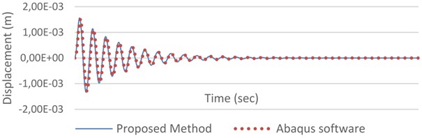
An impact force of 10 kN per 0.01 sec is exerted on the beam at the middle. Damping ratio is assumed to be 0.05. Numerical analysis is adopted by applying Newmark method. Plots of the results, indicate a periodic motion for the point taken at the middle of the beam, Fig. 6. The dynamic behavior of this beam is analyzed in 1000 steps with 0.001 sec time step size. This proposed, and FEM methods are adopted by applying MATLAB and Abaqus software’s, respectively. By comparing the responses, a maximum error of 7 % is observed, which is below 0.1 mm.

Fig. 8Displacement of the cracked beam due to impact force at the middle

3.2. Example 2

An aluminum cantilever beam with single crack, tested by Sinha et al. [7], is considered here. They obtained the modal parameters of the beam through the impulse response method, using a small instrumented hammer for excitation and an accelerometer of mass 0.0035 kg to measure the response. The modal test is run on an intact beam and then on the similar beams with a single crack at 275 mm from the left end and varying depths of 4, 8 and 12 mm. The beam is clamped at the left side by longitudinal and rotary springs. Springs’ stiffness consist of $k_t=$ 26.5 MN/m and $k_{\theta }=$ 150 kNm/rad, Fig. 9. The details of the geometric dimensions and material properties are tabulated in Table 2.

Fig. 9Cantilever beam of example 2 [7]

The natural frequencies obtained for this cracked beam, by applying this proposed method, are in close agreement with those measured by Sinha et. al. [7] through experimental tests, Table 4. The maximum error occurs in the first mode of the first scenario and is equal 1.6 %.

Table 4Comparison of proposed and Sinha et. al. [7] methods

	Frequency of four primary modes in three different damage scenarios
	Scenario 1			Scenario 2			Scenario 3
	${}_{}{}^{*}\eta L=$ 275 mm, $1-\beta =$ 0.16			$\eta L=$ 275 mm, $1-\beta =$ 0.32			$\eta L=$ 275 mm, $1-\beta =$ 0.48
	New method	Measured [7]	% Err	New method	Measured [7]	% Err	New method	Measured [7]	% Err
1	19.680	20	1.6	19.460	19.750	1.46	19.273	19	1.44
2	123.692	124.25	0.4	122.839	124.063	0.99	122.131	123	0.71
3	340.803	340.813	0	335.726	336.875	0.34	331.726	326.563	1.58
4	668.699	662.813	0.89	662.016	662.313	0.86	667.462	660.313	1.08
${}_{}{}^{*}\eta L$: Crack location

3.3. Example 3

A two bay, two storey frame that is studied by Labib et al. [19] is considered here, Fig. 10. The frame specifications are tabulated in Table 2. Two different damage scenarios with a single crack are considered. Different cases for the crack location and depth, together with the corresponding first four natural frequencies are tabulated in Table 5.

Each node of the frame, with three degrees of freedom, has two translations and one rotation. The stiffness terms of the members connected at the node are added together to form the global stiffness matrix of the frame. The natural frequencies are then calculated for the frame. The above process is programmed through MATLAB. The results reported by Labib et al. [19] and those obtained through this proposed method are compared in Table 5. The cracks are assumed to remain open during the whole process.

The dynamic stiffness matrices for this frame, is obtained through this newly proposed method.

Fig. 10Two storey, two slab frame of example 3 [19]

Table 5Comparison of the proposed and Labib et al. [19] methods

Frequency of four primary modes
	Healthy structure			Scenario A, crack depth: 0.2 $H$, $\eta Lc=$ 0.72 m			Scenario B, crack depth: 0.4 $H\eta Lb=$ 2.91 m
Mode	Present	Labib	% Err	Present	Labib	% Err	Present	Labib	% Err
1	3.2676	3.2676	0.003	3.2535	3.2528	0.02	3.2668	3.2674	0.02
2	10.8551	10.8528	0.021	10.8372	10.8346	0.02	10.8512	10.8510	0.002
3	12.0902	12.0841	0.050	12.0823	12.0763	0.05	12.0556	12.0690	0.11
4	14.3223	14.3204	0.083	14.3317	14.3200	0.08	14.1148	14.2237	0.76

3.4. Example 4

A two bay, one storey frame with multiple cracks studied by Labib et al. [18] is considered here, Fig. 11. The beams and columns are of the same $L=$ 12.00 m length. The frame specifications are tabulated in Table 2. Each column is cracked at both the ends that is similar to damages that occur at seismic collapse. Each node of the frame, with three degrees of freedom, has two translations and one rotation. The first five natural frequencies of the frame, for the undamaged and the two other damaged scenarios are tabulated in Table 6. The natural frequencies obtained by this proposed method match the values reported by Labib et al. [18], with the insignificant error below 1 %, Table 6. The cracks are assumed to remain open during the whole process.

Fig. 11Two bay, single story frame of example 4 [18]

Table 6Comparison of the proposed and Labib et al. [18] methods

Frequency of four primary modes
Mode	Healthy structure			Scenario i, Crack depth: 0.2 $H$			Scenario ii, Crack depth: 0.4 $H$
	Present	Labib	% Err	Present	Labib	% Err	Present	Labib	% Err
1	0.5987	0.5987	0	0.5868	0.5916	0.8	0.5719	0.5771	0.90
2	2.4664	2.4667	0.012	2.4518	2.4554	0.15	2.4290	2.4335	0.19
3	3.1085	3.1095	0.032	3.0946	3.0952	0.02	3.0689	3.0693	0.68
4	4.1895	4.1894	0.002	4.1544	4.1539	0.01	4.0936	4.0847	0.20
5	4.5099	4.5085	0.031	4.4625	4.4617	0.001	4.3767	4.3637	0.30

4. Sensitivity analysis

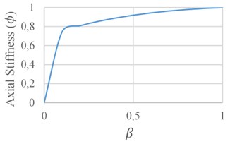
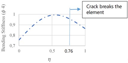
Sensitivity of the Axial (𝜙), Shear (𝜙1), and Bending (𝜙4) stiffness components to the crack severity and its location is analyzed here, Figs. 12 to 14. In Figs. 12(a) to 14(a), the crack location ratio (${\eta }_n$) is assumed to be 0.1, while the effective crack length ratio (${\xi }_n$) is calculated through Eq. (2). In Figs. 12(b) to 14(b), the crack depth ratio ($1-{\beta }_n$) is assumed to be 0.3, while the effective crack length ratio of (${\xi }_n$) is calculated through Eq. (2). Based on Eq. (2) when $1-\beta$, is 0.3,$\mathrm{}{\xi }_n$ becomes 0.2443, therefore when $\eta$ exceeds 0.7557, crack breaks the element boundary and the results are invalid. In this case, the alternative is to move the nodes of the model in a direction until the crack effective length is contained within the single element. In all cases, when the crack depth exceeds 0.8$H$, a sudden reduction occurs, and the element becomes instable. The minimum stiffness reduction occurs when the crack is located near the middle of the element.

According to Fig. 12(a), the axial stiffness reduction is within 0-20 % when the crack depth is within 0 %-80 %. For a crack depth of 50 % a reduction of 8 % occurs. The axial stiffness is not sensitive to the crack location, Fig. 12(b).

According to Fig. 13(a), variation of crack depth from zero to 0.5$H$, leads to a shear stiffness reduction from zero to 14 %. In Fig. 13(b), in situations where the crack is at the ends of the element limits, maximum reduction occurs at the shear stiffness, which reaches to 15 % at a crack depth ratio of 0.3.

Fig. 12Axial stiffness variations: a) in terms of damage severity, b) in terms of damage Location

a)

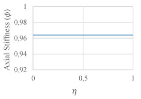
b)

Fig. 13Shear stiffness variations: a) in terms of damage severity, b) in terms of damage location

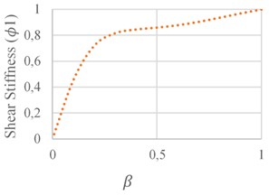
a)

b)

Fig. 14Bending stiffness variations: a) in terms of damage severity, b) in terms of damage location

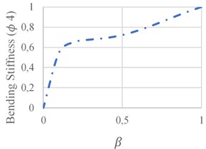
a)

b)

Based on Fig. 14(a), the variation of crack depth from zero to 0.5$H$, leads to bending stiffness reduction from zero to 28 %. In Fig. 14(b) where the crack is close to element boundary, the maximum reduction of 18 % occurs.

5. Conclusions

The methodology proposed in this article is contributive in more parametric analysis of damaged structures. Applying the model reduction of static condensation approach, crack sides’ DOFs are condensed and a new six by six-stiffness matrix is introduced for the first time in this field. Each component of the obtained stiffness matrix is divided by its relevant component of the intact element that yields seven dimensionless coefficients. By applying these coefficients, the sensitivity analysis of stiffness matrix to crack parameters is run in a more accurate, simple and fast manner. Low sensitivity of axial stiffness, moderate sensitivity of shear stiffness, and relatively high sensitivity of bending stiffness to the crack parameters constitute the findings in this study. The crack depth of 0.5$H$, leads to a reduction of 28 %, 14 %, and 8 % for bending, shear, and axial stiffness, respectively. When the crack depth exceeds 0.8$H$, a sudden reduction in stiffness coefficients occurs and the element becomes instable. Shear and bending stiffness reduction varies in different crack location. When the crack is close to element boundaries, maximum reduction occurs in shear and bending stiffness matrix.