Abstract
Aiming to achieve the bearing remaining life prediction, this research proposed a method based on the weighted complex support vector machine (SVM) model. Firstly, the features are extracted by time domain, time-frequency domain method, so as the extract the original features. However, the extracted original features still with high dimensional and include superfluous information, the multi-features fusion technique principal component analysis (PCA) is used to merge the features and reduce the dimension. And the bearing degradation indicator is constructed based on the first principal component, which can indicate the bearing early failure state precisely. Then, based on the life condition indicator, the weighted complex SVM model is used to achieve the bearing remain life prediction, in this model, the particle swarm algorithm (PSO) method is used to select the SVM internal parameters, the phase space reconstruction algorithm is used to determine the structure of the SVM. Cases of actual were analyzed, the results proved the effectiveness of the methodology.
1. Introduction
Bearings are widely used in railway vehicles, automobile, aircraft, and so on. Their failure rate is high and their operation directly affects the overall performance of mechanical equipment. Therefore, accurate and effective condition monitoring and remaining life prediction for bearings have great significance for improving work efficiency, reducing operating costs, and protecting the operation safety.
In order to achieve the bearing condition monitoring and remaining life prediction, there have two key issues. Firstly, how to construct an effective degradation indicator, which need to take advantage of a variety of information and descript the bearing degradation trend and failure point precisely. Secondly, based on the indicator, we need a useful prediction model to achieve the remaining life prediction [1].
In many research, the Kurtosis, RMS and peak indicator are usually being used as the machinery recession indicator. For example: Huang [2] used the Kurtosis and RMS to extract the ball bearing features and indicate the bearing working station. However, the Kurtosis and RMS are not sensitive to the machinery equipment early defect detection. Gebraeel [3] used the failure frequency and the amplitude of the former sixth-order harmonics as the indictor for bearing remaining life prediction. But the FFT analysis results often tend to average out transient vibrations and thus do not provide a wholesome measure of the bearing health status, so it is not suitable been used as the indicator. Liao [4] constructed the PH model and the Logistic model to assess the state of the bearing. Chen [5] established the bearing degradation indictor based on the lifting wavelet package and the fuzzy c-means clustering model. Hong [6] proposed based on the EMD-SOM method to processed the original features and get the indictor. Zhang [7] used the phase space reconstruction to build the trajectories. Those indictors showing the researcher are trying to find a useful indictor to reflect the equipment working condition. However, those indictors mainly based on single indictor which cannot contain the complex and enrich working condition, they also can’t work as a key point to reflect the bearing early failure point. So it is necessary to merge the multiple features and weight to achieve the spatial characteristics comprehensive summery so as to find an effective indictor.
There are many spatial characteristics comprehensive summery method can achieve the merge, such as the principal component analysis (PCA) [8], kernel principal component analysis (KPCA) [9], manifold learning [10]. For example: Yu [11] using the manifold learning method LPP established a bearing recession indictor, but how to select the parameter of LPP have not a unified approach yet. In this research the PCA method is used to construct the indictor. The PCA method have the character of better spatial mapping and integration, it is more stable and do not need to select the parameters. The first principal component of the PCA can weight every character and get the main feature characteristic with minimal information.
Neural network (NN) and the support vector machine (SVM) are the most used artificial intelligence prediction models recently, Tian [12] established a residual life prediction model based on NN method, the author claimed that the model can effectively predict the bearing remaining life based on the collected failure data and the test end data. Du [13] proposed a bearing remaining life prediction model based on NN model. Heng [14] researched the reliability of the bearing based on the NN model, and in the end, the author tried to predict the remaining life of bearing. Mahamad [15] proposed a remaining life prediction model based on the NN method, the RMS and Kurtosis are worked as the inputted features, and the NN model is corrected continuous to improve the forecast accuracy. Farzaneh [16] proposed the grinding mill liners remaining life prediction method based on the ANN. Jaouher [17] proposed the use the Weibull distribution and artificial neural network to achieve the bearing remaining life prediction. However, the fitness function of the neural network method is based on the mean square error between the actual output and the expected output, so in order to get a higher fitness value, the model may fall into “over-learning” or “less-learning” and may even fall into local minimum, this will destroy the stability of the model, and will make the prediction result different. The SVM model is another artificial intelligent technique been used in remaining life prediction. Sun [18] used the SVM established a bearing remaining life prediction model, the author claimed that the model can get a better prediction accuracy than other methods. Caesarendra [19] established a prediction model based on the SVM, and the Kurtosis is used to train the model in the research. Zhao [20] used the SVM constructed a bearing recession prediction model. Widodo [21] constructed the beating remaining life prediction model. Nieto [22] proposed to use the PSO-SVM-based method to achieve the forecasting of the remaining useful life for aircraft engines and evaluation of its reliability. Benkedjouh [23] used the support vector regression model to achieve the bearing remaining useful life estimation. The SVM model is better than NN even when there are only a small number of samples. However, the prediction performance of SVM depends on the setting of a number of parameters that influence the effectiveness of the training stage during which the SVM is constructed based on the available data set. The problem of choosing the most suitable values for the SVM parameters can be framed in terms of an optimization problem aimed at minimizing a prediction error. In this work, this problem is solved by particle swarm optimization (PSO), a probabilistic approach based on an analogy with the collective motion of biological organisms. In addition, in order to determine how many essential observations (inputs) are used for forecasting the future value, the phase space reconstruction method is used to determine the structure of the SVM.
This paper is organized as follows. The methods of signal processing are introduced in Section 2. The SVM model is described in Section 3. The proposed method for bearing remaining life prediction is described in Section 4. The case study is presented in Section 5, in which the proposed method is validated. Finally, the conclusions are given in Section 6.
2. Signal processing
In this section, the feature extraction methods time domain, frequency domain, and time-frequency domain are discussed. The sixteen-time domain statistical characteristics (feat1-feat16) and twelve frequency domain statistical characteristics (feaf1-feaf12), for a total of twenty-eight feature parameters are extracted based on the methods as shown in Tables 1 and 2, respectively. Parameters feat1-feat10 were extracted because they can reflect the vibration amplitude and energy in the time domain. Parameters feat11-feat16 were extracted because they can represent the time series distribution of the signal in the time domain. Parameter feaf1 were extracted because they can indicate the vibration energy in frequency domain. Parameters feaf2-feaf4, feaf6-feaf7, feaf11-feaf12 were extracted because they can describe the convergence of the spectrum power. Parameters feaf5, feaf8–feaf10 were extracted because they can show the position change of the main frequencies.
Table 1The time domain characteristic features
The characteristic features | The characteristic features |
is a signal series for , is the number of collected data points. represents the Skewness which is calculated in , and the represents the Kurtosis which is calculated in . | |
There are some most usually used time-frequency methods, such as: short-time Fourier transform(STFT), wavelet, empirical mode decomposition (EMD). This time-frequency domain analysis used time-frequency distributions to reveal fault patterns they were also used to provide how the frequency changes with time. But the disadvantage of wavelet analysis is its non-adaptive nature. Once the basic wavelet is selected, one will have to use it to analyze all the data. The disadvantage of STFT is how to select the suitable analysis window function, if the analysis window function is not appropriate, the frequency information will leak. In this research, the EMD is used to extract the typical features. The advantage of EMD is the presentation of signals in time-frequency distribution diagrams with multi-resolution, during which choosing some parameters is not needed. The EMD energy can represent the characteristic of vibration signals, and thus is used as the input features. The first six intrinsic mode function (IMF) energy data sets were chosen as the original features.
Table 2The frequency domain characteristic features
The characteristic features | The characteristic features |
is a spectrum for , is the number of spectrum lines; is the frequency value of the th spectrum line | |
The feature extraction method PCA is used to fuse the relevant useful features and extract the more sensitive features to work as a recession indictor of the bearing. The procedure of feature extraction and life recession indictor construction can be described as follow:
1) Use the time domain analysis methods and frequency domain analysis methods to extract the statistical features;
2) Use the energy of the first six IMF components to get the features of the bearing at each time;
3) Use the PCA to reduce the original features dimensions and extract the first principal component.
Setting up the features extracted in step 1 and 2 can be expressed as:
while the , represents the value of the features.
Through the PCA analysis we can get that the linear combination of features , ,…, can be expressed as:
where meet the need that , 1, 2,…,, the and () independent of each other; get the max variance of all linear combination of Eq. (2). Then the can catch the most typical features in this research and been used as the recession indictor.
3. The SVM model for remaining life prediction
3.1. SVM prediction model
SVM is a machine learning tool that uses statistical learning theory to solve multi-dimensional functions. It is based on structural risk minimization principles, which overcomes the extra-learning problem of ANN.
The learning process of regression model LS-SVM is essentially a problem in quadratic programming. Given a set of data points (,)…(,) such that as input and as target output, the regression problem is to find a function such as Eq. (3):
where is the high dimensional feature space, which is nonlinear mapped from the input space . is the weight vector, the bias [24].
After training, the correspondingcan be found through for the outside the sample. The-support vector regression (-SVR) by Vapnik controls the precision of the algorithm through a specified tolerance error. The error of the sample is , regardless of the loss, when ; else consider the loss as . First, map the sample into a high dimensional feature space by a nonlinear mapping function and convert the problem of the nonlinear function estimates into a linear regression problem in a high dimensional feature space. If we let be the conversion function from the sample-space into the high dimension feature space, then the problem of solving the parameters of is converted to solving an optimization problem Eq. (4) with the constraints in Eq. (5):
The feature space is one of high dimensionality and the target function is non-differentiable. In general, the LS-SVM regression problem is solved by establishing a Lagrange function, convert this problem to a dual optimization, i.e., problem Eq. (6) with constraint of Eq. (7) in order to determine the Lagrange multipliers , :
where , are Lagrange multipliers and, . . evaluates the tradeoff between the empirical risk and the smoothness of the model.
The LS-SVM regression problem has therefore been transformed into a quadratic programming problem. The regression equation can be obtained by solving this problem. With the kernel function , the corresponding regression function is provided by Eq. (8):
where the kernel function is an internal product of vectors and in feature spaces and .
3.2. The LS-SVM model parameters selection
The particle swarm optimization algorithm was first proposed in 1995. It is an optimization method based on a set of particles whose coordinates are potential solutions in the search space. Particles in PSO will change their coordinates (their solutions) by migrating. During migrating, each particle adjusts its own coordinates based on its own past experience and other particles’ past experiences.
The PSO was chosen to optimize selected the SVM parameters through the following formula:
where the subscript represents the th particle. represents the -dimensional.
The subscript represents thegeneration. is the velocity of the th particle in the th iteration; is the position of the th particle; is the pbest position of the th particle; is the gbest position (pbest represents the local optimum of the particles, gbest represents the overall situation optimum of the particles); The represents the inertia weight. , are learning factors. , represent two independent random functions.
The root-mean square error (RMSE) is used as the criteria to evaluate the proposed algorithm accuracy:
where represents the total number of data points in the test set, is actual value in training set or test set, and represents the predicted value of the model.
The process of optimizing the parameters , based on the PSO is given below:
(1) At the beginning of the optimization process, randomly initialize population size, , , , , , determine the termination condition, positions and velocities of the particle, mapping the LS-SVM parameters , into a group of particles, initialize the initial position of each particle, pbest, gbest of the particles;
(2) When training the SVM, using the Eq. (11) as the PSO fitness function;
(3) Use the target parameters , as the particles, use their initial values as the SVM parameters in step 2), the corresponding value of the fitness function as the optimal solution of the , ;
(4) Use the initial error value of step 2) as the particle’s initial fitness value, search the optimal value as the global fitness value among the initial fitness value, and the corresponding particles as the current global optimal solution;
(5) Updating the velocity and position vector;
(6) Re-substituted the updated parameters , into the SVM model, and re-training the SVM model according to the step 2), save the output value, calculate the fitness value of the particles again;
(7) Comparing the saved global fitness value gotten in step (6) with the current particle’s fitness value, if the global fitness value superior to the current particle’s fitness value, update the current particle’s fitness value according to the step (5), and update the current particle’s optimal value equal to the corresponding particle’s optimal value gotten in step (6);
(8) While the termination conditions are not met, return to step (5);
(9) End loop.
3.3. The prediction strategy and the structure of the SVM model
Traditional forecasting methods mainly achieve single-step prediction, when those methods are used for multi-steps prediction, they can’t get an overall development trend of the series. Multi-steps prediction method has the ability to obtain overall information of the series which provides the possibility for long-term prediction. There are two typical alternatives to build multi-steps life prediction model. One is iterated prediction and the other is direct prediction. The comparison of the two strategies can be found in a number of literatures [25]. Marcellino [26] presented a large-scale empirical comparison of iterated versus direct prediction. The results show that iterated prediction typically outperforms the direct prediction. So, the iterated multi-steps prediction strategy has numerous advantages and will be adopted in this paper.
In order to determine the structure of the SVM, we constructed a three layers SVM prediction model. But, to achieve the multi-steps time series life prediction there is a basic problem should be suppressed. That is how many essential observations (inputs) are used for forecasting the future value (The output node number is 1), so-called embedding dimension . In order to suppressed the problem, the CAO method [27] which is particularly efficient to determine the minimum embedding dimension through the expansion of neighbor point in the embedding space, is employed to select an appropriate embedding dimension . Then, the SVM input node number is determined.
To effective select an appropriate embedding dimension based on the CAO method, the phase space reconstruction method should be mentioned. The fundamental theorem of phase space reconstruction is pioneered by Takens [28]. For an N-point time series , a sequence of vectors in a new space can be generated as: , where , is the length of the reconstructed vector ; is the embedding dimension of the reconstructed state space; and is embedding delay time. The time delay is chosen through the autocorrelation function [29]:
where , is the average value of the time series. The optimal time delay is determined when the first minimum value of occurs.
The embedding dimension is chosen through CAO method, defining the quantity as follows:
where is the Euclidian distance and is given by the maximum norm. means the th reconstructed vector and is an integer, so that is the nearest neighbor of in the embedding dimension . A new quantity is defined as the mean value of all :
is only dependent on the dimension and time delay . To investigate its variation from to 1, the parameter is given by:
By increasing the value of , the value is also increased and it stops increasing when the time-series comes from a deterministic process. If a plateau is observed for , then is the minimum embedding dimension. But has the problem of slowly increasing or has stopped changing if is sufficiently large. CAO introduced another quantity to overcome the problem:
where:
Through CAO method, the embedding dimensionof the SVM prediction model is chosen. The structure of the SVM model is determined.
4. The procedure of the proposed method.
The flowchart of the proposed method is showed in Fig. 1.
Fig. 1The flowchart of proposed bearing residual life prediction method
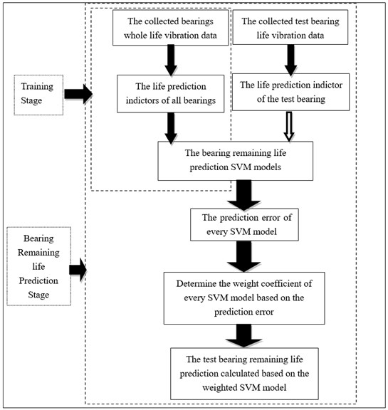
Specific steps are as follow:
(1) Selecting a number of bearings for full life test, and collected the relevant recession data till the bearings failed.
(2) Through the time domain, frequency domain and time-frequency domain features to processed the collected full life test data, so as to obtain the multi-dimension features of every bearing;
(3) Using the PCA to construct the bearing recession indictor, using this indictor as the datum value, and compare the predicted value with the datum value so as to find prediction error.
(4) Although the bearing working in the same condition, however, the bearing work lifes are different, so they got life indictor by every bearing need to be fit and interpolation. In this research, all bearing recession indictor are fitted into the same number of points.
(5) The PSO method is used to select the SVM parameters, the phase space reconstruction algorithm is used to determine the structure of the SVM and the got optimal SVM model are used as the recession models, and the indictors get in step (4) are used to train the SVM models.
(6) Selecting a point in the recession indictor of the test bearing, make sure the working time and index value represented by the point, putted the point into the trained SVM models, get the corresponding output values, compared the output values with the actual value, and got the prediction error of each SVM models. According the prediction error of each model, determined the weighting factor of each model. And finally get the remaining life of the test bearing through Eqs. (19) and (20):
where represents the number of the been trained SVM models, represents the corresponding weight factor of each SVM prediction models, represents the presented time based on each SVM prediction models, represents the weighted summation of presented time based on all SVM models. represents the actual work time of the test bearing model.
5. Validation and application
5.1. Case 1
The vibration signals used in this paper are provided by the Center for Intelligent Maintenance Systems (IMS), University of Cincinnati [30]. The experimental data sets are generated from bearing run-to-failure tests under constant load conditions on a specially designed test rig as shown in Fig. 2. The bearing test rig hosts four test Rexnord ZA-2115 double row bearings on one shaft. The shaft is driven by an AC motor and coupled by rub belts. The rotation speed is kept constant at 2000 rpm. A radial load of 6000 lbs is added to the shaft and bearing by a spring mechanism. A PCB 353B33 high sensitivity quartz ICP accelerometer is installed on each bearing housing. The NI 6062E card is used to collected the vibration data every 10 minutes. The data sampling rate is 20 kHz and the data length is 20,480 points as shown in Fig. 3. Data collection is done using a National Instruments LabVIEW program. Four bearings are used for full time accelerated life test, and 3 bearings recession data were used for training the SVM, getting 3 forecasting models and 1 bearing recession data for prediction.
The Time-domain, frequency domain, time-frequency domain methods are used to deal with the collected vibration data as described in Section 2. The extract features are showed in Figs. 4-6.
Fig. 2The test rig
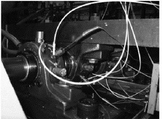
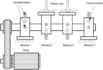
Fig. 3The collected vibration signals
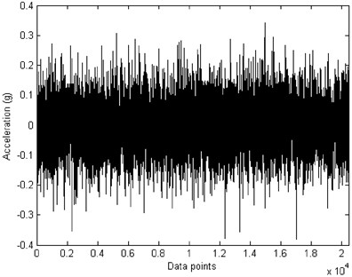
Fig. 4Sixteen indicators of the time domain: a) mean value; b) RMS; c) mean-square-root amplitude; d) absolute value; e) skewness; f) kurtosis; g) variance; h) the maximum value; i) the minimum value; j) the peak-to-peak value; k) index indictor; l) peak-to-peak indictor; m) pulse indictor; n) margin index; o) skewness index; p) kurtosis indicator
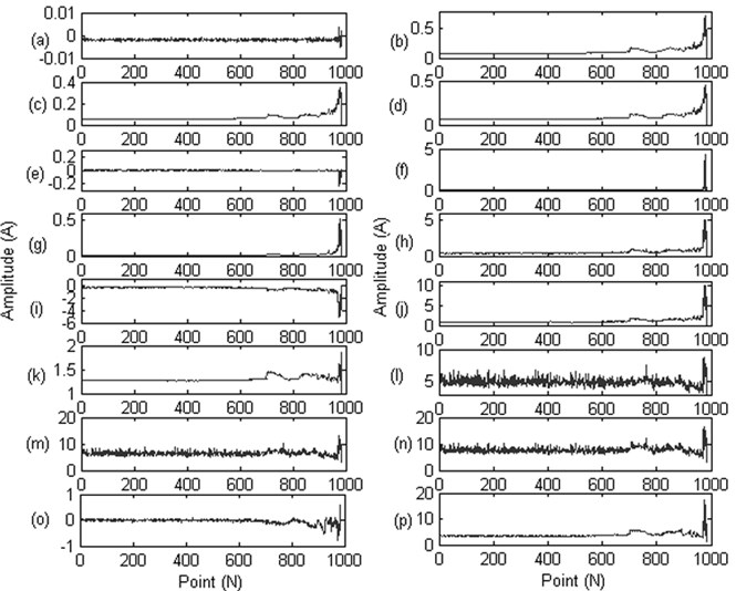
Fig. 5Twelve indicators of the frequency domain: a) the mean frequency; b) frequency standard deviation; c) the frequency characteristics 1; d) the frequency characteristics 2; e) frequency center; f) the frequency characteristics 3; g) RMS frequency; h) the frequency characteristics 4; i) the frequency characteristics 5; j) the frequency characteristics 6; k) the frequency characteristics 7; l) the frequency characteristics 8
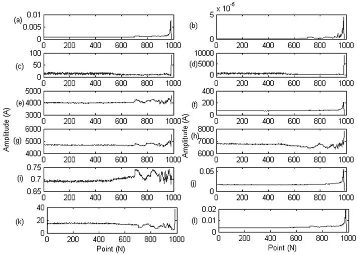
Fig. 6Six IMF energy indicators of the time-frequency domain: a) IMF1 energy indicator; b) IMF2 energy indicator; c) IMF3 energy indicator; d) IMF4 energy indicator; e) IMF5 energy indicator; f) IMF6 energy indicator
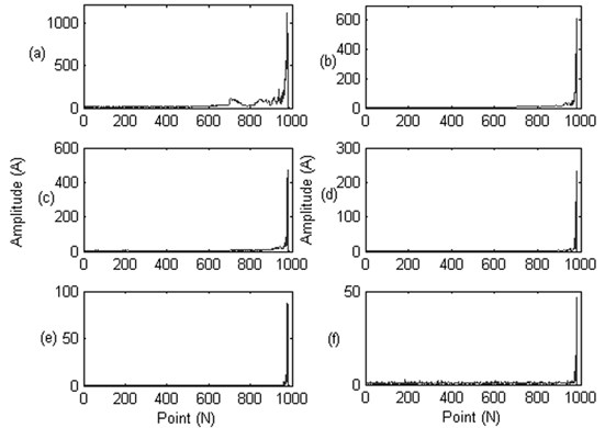
From Figs. 4-6 we can see that, some features are not appropriate to reflect the bearing degradation process, for example, the feature (a), (e) in Fig. 4 still show as a straight line, where (l), (m), (n) features in Fig. 4 contain a lot of noise information, feature (d) in Fig. 5 and feature (e), (f), (g) in Fig. 6 didn’t sensitive to the early fault information. So, we need to extract the typical feature from these original features to better reflect the bearing degradation process,
The PCA is used to reduce the dimensionality of calculated features, in this research, the first principal component is chosen, in order to compare the effect of the recession indictor of the Kurtosis and the PCA, the result is shown in Fig. 7 and Fig. 8.
Fig. 7The kurtosis performance of the life-cycle stage indictor about the measured bearing
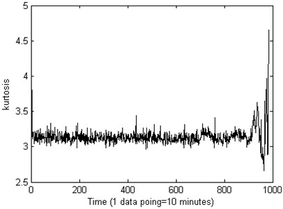
Fig. 8The PCA performance of the life-cycle stage indictor about the measured bearing
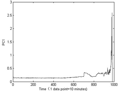
From Fig. 7 we can see that, the Kurtosis is not sensitive to the bearing running fault, especially the early fault, it will on duty until the end of the test bearing life, the Kurtosis showing a fluctuation. From the Fig. 8 we can see that, the machine is in normal condition during the time correlated with the first 700 points. After that time, the condition of the bearing suddenly changes. It indicates that there are some faults occurring in this bearing. Then, though the autocorrelation function method theis set as 36 for PC1 value as shown in Fig. 9.
After determine the delay time, the embedding dimension is selected by the CAO method. The results are shown in Fig. 10, the optimal embedding dimension for PC1, is chosen as 7.
Fig. 9The τ is set as 36 for PC1 value though the autocorrelation function
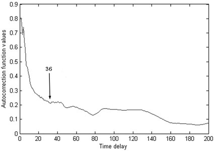
Fig. 10The optimal embedding dimension d is selected by the CAO method
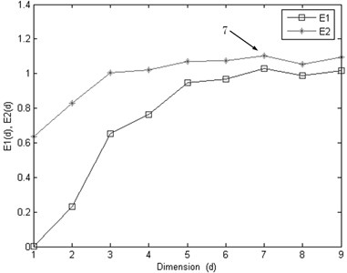
Based on the selected optimal embedding dimension and the delay time, the LS-SVM model is used to achieve the multi-steps prediction. The essential observations (inputs) are used for forecasting the future value is set to 7, the output node number is 1.
The LS-SVM model is used to achieve the multi-steps prediction, the feature of PC1 is used (fitted into 984 points of 4 bearings). The iterated multi-steps prediction strategy is used. The PSO is used to obtain the main parameters of the model, the particle swarm population size is set to 100, the number of the particles is set to 20. The fitness function is set to get the minimum prediction error with the optimized parameters. The prediction error is set to 0.001. The PSO particle’s dimension is set to 2, theis set to 0.5, the is set to 1, the is set to 1, based on the CAO method to determine the embedding dimension number, the LS-SVM model input number is set to 7. The optimized obtain parameters is 90.3, the is 20. Then the two parameters are used to build the LS-SVM model to train and predict the value. The training data length is set to 984 points and the test data point is set to 840 points. The degradation curves and the fitted curve (the fitting number is 5) of the 3 training bearings are showing in Fig. 11. The test beating recession curve and the fitted curve is showing in Fig. 12.
Fig. 11The degradation trend carve of three training bearing: a) the training bearing 1 and its fitted curve; b) the training bearing 1 and its fitted curve; c) the training bearing 1 and its fitted curve
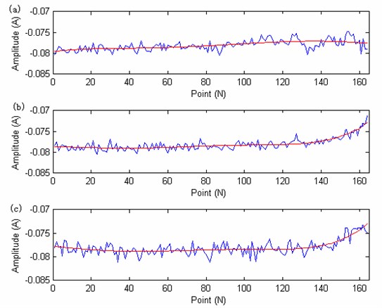
Fig. 12The degradation trend carve of the test bearing
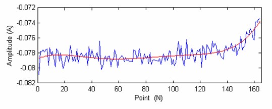
From the Fig. 11 and Fig. 12 we can see that, the recession curve and its fitted curve is similar to the recession curve and fitted curve of training bearing 2, and far away with bearing1, so the SVM prediction model should have a heavy weigh factor than the bearing1. From the Fig. 12 we can see that there are 164 points, the 140 point is chosen for predicting (The remaining life should be 24 point, one point represents the actual work hour). The prediction results are:
The weighted factors of the 3 training bearing are: model 1: 0.0516; model 2: 0.8900; model 3: 0.0584.
The predicted remaining life is 18.3608. The prediction value is closer to the actual value 24, get a good prediction result.
In order to compare the different remaining life prediction methods that are proposed by other lecture, this research achieve a comparison among the proposed methods. 1) The vibration signals is proposed by the EMD energy entropy, and the SOM neural network is used to processed the features, the confidence value model is used to achieve the remaining life prediction [6]. 2) The time series data is processed by the phase space reconstructing method and the weighted Normalized cross correlation model is constructed to achieve the remaining life [7]. 3) The accurate bearing remaining useful life prediction based on Weibull distribution and artificial neural network [17]. 4) The bearing remaining life prediction model is achieved by the Hybrid PSO–SVM-based method [22]. 5) The proposed method in this research. The remaining life prediction results of different methods are showing in Table 3.
Table 3The prediction results of different methods (The actual remaining life value is 24)
The prediction methods | The actual remaining life value |
The SOM model and confidence value [5] | 12.4 |
The phase space reconstructing method and the weighted normalized cross correlation model [6] | 14.8 |
The Weibull distribution and artificial neural network [16] | 13.3 |
The Hybrid PSO–SVM-based method [22] | 14.4 |
The proposed method | 18.3 |
From the result we can see that the neural network and the SVM model are used for the remaining life prediction, however the neural network model are not stable, the result may changed even the parameters are same when constructing the model, the SVM model can work better than the ANN model, however, if only one model is used in remaining life prediction, the result will be affected by the constructed model, so the weighted models are necessary for remaining life prediction, and based on the results, we can see the proposed model work better than the proposed model in other lectures.
5.2. Case 2
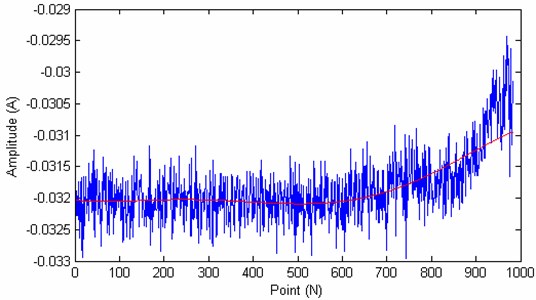
In Case 1, the 4 bearing are working in the same state, they all work in the unified operating conditions. In order to further validate the proposed method, the other data provide also by the Center for Intelligent Maintenance Systems (IMS), University of Cincinnati [28] are used (8 bearing full time recession data) together with the 4 bearing data used in Case1 for validation. In this research the bearing 1 recession indictor of case 1 is used for test, and the remaining 11 bearings recession data are used for training. As can be seen from the Case 1, sine the work condition of the 3 bearing used in Case 1 are very different with the 8 bearings, so the weight factors of the 3 bearing may greater than the 8 bearings. The iterated multi-steps prediction strategy is used. The PSO is used to obtain the main parameters of the model, the particle swarm population size is set to 300, the number of the particles is set to 20. The fitness function is set to get the minimum prediction error with the optimized parameters. The prediction error is set to 0.005. The PSO particle’s dimension is set to 2, the is set to 0.1, the is set to 1, the is set to 1, based on the CAO method to determine the embedding dimension number, the LS-SVM model input number is set to 7. The optimized obtain parameters is 620, the is 511. Then the two parameters are used to build the LS-SVM model to train and predict the value. The recession indictor (Unified interpolated to 984 points) and the fitted curve (the fit number is 5) of 11 training bearing are showing in Fig. 13. There are 984 points, the 440 point is chosen for predicting (The remaining life should be 544 point, one point represents the actual work hour).
The weight factor of every bearing prediction SVM models is: model 1: 0.0048; model 2: 0.0043; model 3: 0.0044; model 4: 0.0034; model 5: 0.0053; model 6: 0.0056; model 7: 0.0039; model 8: 0.0041; model 9: 0.0004; model 10:0.0000; model 11: 0.9638.
The remaining life of the test bearing 1 is 559.2252. From the got result we can see that the proposed method can get the remaining life 544 of the bearing precisely, which validate the useful of the proposed method.
However, from the results of Case 1 and Case 2 we can also get that, in order to get a more accurate prediction result, the collected data must be representative, and the working condition of the test bearing must be similar with the training bearing, the prediction result can be precisely.
Fig. 13The degradation trend curves of eleven training bearing: a) the bearing degradation trend curve of bearing 1 (new added); b) the bearing degradation trend curve of bearing 2 (new added); c) the bearing degradation trend curve of bearing 3 (new added); d) the bearing degradation trend curve of bearing 4 (new added); e) the bearing degradation trend curve of bearing 5 (new added); f) the bearing degradation trend curve of bearing 6 (new added); g) the bearing degradation trend curve of bearing 7 (new added); h) the bearing degradation trend curve of bearing 8 (new added); i) the bearing degradation trend curve of bearing 1 (go in case 1); j) the bearing degradation trend curve of bearing 2 (go in case 1); k) the bearing degradation trend curve of bearing 3 (got in case 1)
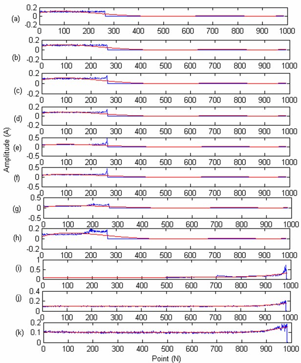
Fig. 14The degradation trend carve of the test bearing
6. Conclusions
1) Aiming at the problem that the bearing degradation process indicator is very difficult to been built. This paper constructs the indicator based on the principal component analysis weighted fusion method. The time domain, frequency domain and time-frequency domain feature information extraction methods, explores the spatial distribution of these features. Constructs the indicator based on the data space mapping and weight fusion method, the results show that the constructed indicator can reflect the bearing degradation trend effectively.
2) Aiming at the traditional life prediction method can’t predict the bearing remaining life effectively, this article uses the optimal SVM to achieve. Uses the phase space reconstruction method to select the input parameters of the SVM, uses the particle swarm algorithm to select the SVM internal parameters. Through the recession indictor to train the SVM models and get the weight factor, based on the weight factor of every SVM model to achieve the bearing life remaining life prediction, results proved the effectiveness of the proposed method.
References
-
Yang W. X., Court R. Experimental study on the optimum time for conducting bearing maintenance. Measurement, Vol. 46, Issue 8, 2013, p. 2781-2791.
-
Huang R. Residual life predictions for ball bearings based on self-organizing map and back propagation neural network methods. Mechanical Systems and Signal Processing, Vol. 21, 2007, p. 193-207.
-
Gebraeel N., Lawley M., Liu R. Residual life predictions from vibration-based degradation signals: a neural network approach. IEEE Transactions on Industrial Electronics, Vol. 51, 2004, p. 694-700.
-
Liao H. T., Zhao W. B., Guo H. R. Predicting remaining useful life of an individual unit using proportional hazards model and logistic regression model. Annual Reliability and Maintainability Symposium, 2006, p. 127-132.
-
Pan Y. N., Chen J., Xing L. L. Bearing performance degradation assessment based on lifting wavelet packet decomposition and fuzzy c-means. Mechanical Systems and Signal Processing, Vol. 24, 2010, p. 559-566.
-
Hong S., Zhou Z. An adaptive method for health trend prediction of rotating bearings. Digital Signal Processing, Vol. 35, 2014, p. 117-123.
-
Zhang Q., Wai-Tat Tse P., Wan X. Remaining useful life estimation for mechanical systems based on similarity of phase space trajectory. Expert Systems with Applications, Vol. 42, 2015, p. 2353-2360.
-
Dong S. J., Luo T. H. Bearing degradation process prediction based on the PCA and optimized LS-SVM model. Measurement, Vol. 46, 2013, p. 3143-3152.
-
Yang W. X., Peter W. T. Development of an advanced noise reduction method for vibration analysis based on singular value decomposition. NDT&E International, Vol. 36, 2003, p. 419-432.
-
Yan W., Zhang C. K., Shao H. H. Nolinear fault diagnosis method based on kernel principal component analysis. High Technology Letters, Vol. 11, Issue 2, 2005, p. 189-192.
-
Yu J. B. Bearing performance degradation assessment using locality preserving projections and Gaussian mixture models. Mechanical Systems and Signal Processing, Vol. 25, 2011, p. 2573-2588.
-
Tian Z. G., Wong L., Safaei N. A neural network approach for remaining useful life prediction utilizing both failure and suspension histories. Mechanical Systems and Signal Processing, Vol. 24, 2010, p. 1542-1555.
-
Du S. C., Lv J., Xi L. F. Degradation process prediction for rotational machinery based on hybrid intelligent model. Robotics and Computer-Integrated Manufacturing, Vol. 28, 2012, p. 190-207.
-
Heng A., Tan Andy C. C., Joseph Mathew Intelligent condition-based prediction of machinery reliability. Mechanical Systems and Signal Processing, Vol. 23, 2009, p. 1600-1614.
-
Mahamad A., Saon S., Hiyama T. Predicting remaining useful life of rotating machinery based artificial neural network. Computers and Mathematics with Applications, Vol. 60, 2010, p. 1078-1087.
-
Ahmadzadeh F., Lundberg J. Remaining useful life prediction of grinding mill liners using an artificial neural network. Minerals Engineering, Vol. 53, 2013, p. 1-8.
-
Ben Ali J., Morello B., Lotfi Saidi Accurate bearing remaining useful life prediction based on Weibull distribution and artificial neural network. Mechanical Systems and Signal Processing, Vol. 56, 2015, p. 150-172.
-
Sun C., Zhang Z. S., He Z. J. Research on bearing life prediction based on support vector machine and its application. 9th International Conference on Damage Assessment of Structures (DAMAS 2011), Journal of Physics: Conference Series, Vol. 305, 2011, p. 12-28.
-
Caesarendra W., Widodo A., Yang B. S. Combination of probability approach and support vector machine towards machine health prognostics. Probabilistic Engineering Mechanics, Vol. 26, 2011, p. 165-173.
-
Zhao F., Chen J., Xu W. Condition prediction based on wavelet packet transform and least squares support vector machine methods. Additional services and information for Proceedings of the Institution of Mechanical Engineers, Part E: Journal of Process Mechanical Engineering, Vols. 71-79, 2008.
-
Widodo A., Yang B. S. Machine health prognostics using survival probability and support vector machine. Expert Systems with Applications, Vol. 38, 2011, p. 8430-8437.
-
García Nieto P. J., García-Gonzalo E., Sánchez Lasheras F. Hybrid PSO-SVM-based method for forecasting of the remaining useful life for aircraft engines and evaluation of its reliability. Reliability Engineering and System Safety, Vol. 138, 2015, p. 219-231.
-
Benkedjouh T., Medjaher K., Zerhouni N. Remaining useful life estimation based on nonlinear feature reduction and support vector regression. Engineering Applications of Artificial Intelligence, Vol. 26, 2013, p. 1751-1760.
-
Ioannides E., Harris T. A. A new fatigue life model for rolling bearing. ASME Journal of Tribology, Vol. 107, 1985, p. 367-378.
-
Tran V. T., Yang B. S., Tan A. C. C. Multi-step ahead direct prediction for the machine condition prognosis using regression trees and neuro-fuzzy systems. Expert Systems with Applications, Vol. 36, 2009, p. 9378-9387.
-
Marcellino M., Stock J., Watson M. W. A comparison of direct and iterated multi-step AR methods for forecasting macroeconomic time series. Journal of Econometrics, Vol. 135, 2006, p. 499-526.
-
Cao L. Practical method for determining the minimum embedding dimension of a scalar timeseries. Physica D, Vol. 110, 1997, p. 43-50.
-
Taken F. Detecting Strange Attractors in Turbulence. Dynamical Systems and Turbulence, Springer, New York, 1981, p. 366-381.
-
Fraser A. M., Swinney H. L. Independent coordinates for strange attractors from mutual information. Physical Review A, Vol. 33, 1986, p. 1134-1140.
-
IMS Bearings Data Set, http://ti.arc.nasa.gov/tech/dash/pcoe/prognostic-data-repository/, 2014.
Cited by
About this article

This research is supported by the National Natural Science Foundation of China (No. 51405047,51305472), The Scientific Research Fund of Chongqing Municipal Education Commission (No. KJ1500529), Chongqing Postdoctoral Science Foundation Funded Project (No. xm2015001), Science Application Research Project of COSCO, China (Grant No. 2010-1-H-001), The Key Laboratory of Road Construction Technology and Equipment (Chang’an University), (No. 2014SZS11-K02). The Basic and Advanced Research Key Project of Chongqing. (No. cstc2015jcyjBX0140). The authors are grateful to the anonymous reviewers for their helpful comments and constructive suggestions.
Shaojiang Dong make the contribution of the whole article, he decides the research method, and also make the test been validated. Jinlu Sheng, make the contribution of the bearing life prediction model, he mainly does the model setting up research, and he also do some test work. Zhu Liu make the contribution of the bearing fault test, he analysis the bearing degradation signal and give some conclusion. Li Zhong, make contribution to the article in the bearing performance analysis, based on the research, we can clear the bearing working condition. Hanbing Wei make contribution to the bearing life weight index research, include the research, we put the method in the research for bearing life prediction.
