Thorax measurement and analysis using electrical impedance tomography

1. Introduction

Recently a lot of attention was focused on utilization of the Electrical Impedance Tomography (EIT) in medical care. EIT is a technique of visualizing interior of an object based on electrical measurements made on the surface. Although there are already other well-established techniques like a magnetic resonance imaging (MRI) or a computed tomography (CT) they are both not suitable for a real-time monitoring at the bedside. Moreover, EIT offers less expensive, non-ionizing approach. The main drawback of EIT is mainly that it provides images which are blurred and have spatial resolution lower than MRI or CT. The spatial resolution is at best limited approximately by the distance between electrodes.

In medicine EIT can be generally used for phenomena where an impedance change over time is encountered. For example, a successful bladder filling [1] surveillance, a stomach gastric emptying [2] and of course lung ventilation [3] and a cardiac perfusion [4] in the area of thorax is reported. In this report we will focus on imaging of ventilation and perfusion [5].

There are basically two types of EIT: absolute and difference. The absolute one is very vulnerable to mismatch in electrode positioning, not exactly specified geometry of the measured object or inaccurately known contact impedance. This concept is for the time being developed mainly on phantoms although few measurements on real targets were already made [6]. On the other hand, to circumvent such problems a difference measurement can be made when a reference is taken at the begging of the measurement. This is clearly unsuitable for thoracic measurements. To overcome such a limitation of difference imaging a concept of an average impedance over a certain time window as a reference [3] was proposed or computation of local standard deviations at each pixel and plotting them at the corresponding image position [3] was used. In this paper we tried another approach of taking reference during a deep expiration of a subject.

The main objective of EIT imaging of thorax is nowadays an individual and real-time adjustment of mechanical ventilation for patients with problems with breathing such as acute respiratory distress syndrome (ARDS) [7, 8].

2. Materials and methods

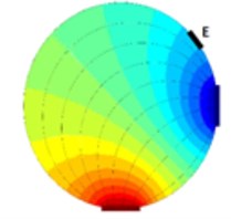
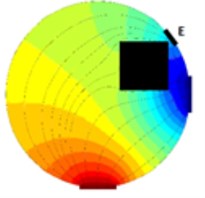
As it is visible from previous section EIT is a promising way of reconstructing cross-sectional slices of an object based on boundary measurements. EIT is in fact a device which consists from a precise current source and a very accurate voltmeter. The electrodes on the boundary of a vessel (or a human body in our case) are driven by the current source (one electrode is a source and a different one is a sink) and the voltage measurements are made on the remaining electrodes (Fig. 1). Clearly when an object is inserted to the test vessel which was not there while taking reference (Fig. 1(a)) the voltage at the electrode E (Fig. 1(b)) differs from the voltage taken at the time of taking the reference.

There is also an approach when several electrodes are driven at the same time [9] but this one is rarely used (this approach delivers very precise measurements which can be then used even for absolute imaging) because it is very complex. There are many modifications of tomographic systems. They usually differ in the hardware used and sensing strategy.

Fig. 1Principle of voltage changes on an arbitrary electrode E, a) vessel with fluid, b) a square cross-sectional object is inserted into the vessel with fluid.

a)

b)

2.1. Sensing strategy

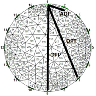
The most common system in use is using Sheffield strategy (adjacent) when adjacent electrodes are driven by current and at the same time different adjacent electrodes are measured for the difference induced voltage. For a system with one plane and 16 electrodes (this system will be considered in this paper) this results for total of 104 independent measurements. This was the first successful system and because of historical reasons the system is still widespread even though it was shown that other strategies exercise inherently better results [10]. From [10] it follows that the best measurement strategy is stimulation and sensing in a way when electrodes are nearly opposite but not exactly opposite. This strategy is also called [1 7] strategy or “skip 5” (electrodes 1 and 7 are driven by current and electrodes 2 and 8 are sensed etc.). Nevertheless, we have examined all three often discussed strategies in our experiment to verify the best method. A circular test vessel was filled with tapped water and on the bed of the vessel was thick sediment of sand. At this point we took a reference of the measuring plane above the sediment and started to turn the vessel upside down. Two positions were selected for taking a measurement: the first one when sand formed at the sensing plane small deposit (Fig. 2 – first row) and the second one when the sand filled nearly the whole area of the sensing plane (Fig. 2 – second row). Results after FEM processing are visible in Fig. 2(a, d) for adjacent strategy, in Fig. 2(b, e) for opposite strategy and in Fig. 2(c, f) for [1 7] strategy. It is visible that adjacent strategy reliably represents a real scenario, opposite stimulation (pattern [1 9]) and sensing have problems with mirroring the object (the images are axial symmetric) and finally the so-called optimal strategy (pattern [1 7]) does not correspond to the real scenario. Based on this experiment we have decided to use traditional adjacent strategy further on since it provided by far the most reliable results.

In the case of adjacent and optimal pattern there are 104 measurement whereas for opposite there are only 28 measurements.

The main EIT advantages (compared to most common computer tomography – CT – scans) are mainly: low cost, high acquisition frequency, small size and non-ionizing approach. The drawback of EIT which is low spatial resolution is caused mainly by the fact of badly-posed problem [11] because of inevitable errors during measurement and due to quantization.

Fig. 2Comparison of results from different stimulation and sensing strategies; a) and d) adjacent, b) and e) opposite and c) and f) optimal [1 7], the first row corresponds to small deposit of sand and the second row corresponds to large deposit of sand at the level of sensing plane

a)

b)

c)

d)

e)

f)

3. Results and discussion

There were many attempts to introduce the EIT methodology into clinical applications. One of them is for example designing an active electrode belt for the sake of ease of placing electrodes and minimizing errors [15]. Also, several rather experimental measurements of thorax were reported for pigs and even for humans Anyway monitoring lungs is very challenging because it is not possible to use the differential approach. The main advantage of the differential approach is that it minimizes the effect of contact impedances of electrodes and to certain level also minimizes not precisely located electrodes.

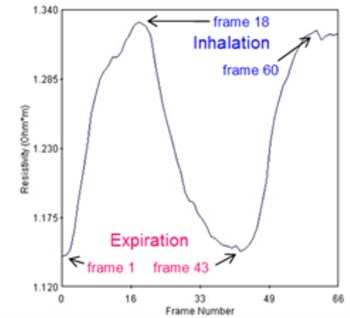
For the case of lungs, it is impossible to take the reference and hence using true differential approach. Regardless of this we have used “pseudo-differential” approach – see [15]. In our case the volunteer has strived to exhale as much air as possible and at that moment we have taken a reference. Then during the measurement, the volunteer has taken deep breath for two times and in between he again exhaled as much as possible. A commercial p2+ EIT system from ITS, England was used. The average resistivity measured across all the calculated data points in the cross section is visible from Fig. 3(a). The graph can be used for estimation of end-expiratory lung volume (EELV) from end-expiratory lung impedance (EELI). It was proven that a linear dependence exists between EELI and EELV [16].

Fig. 3a) Average resistivity measurements for a volunteer exhaling as much as possible and taking deep breath, b) electrode assignment for 16-electrode system

a)

b)

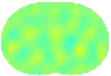
The results using 1-norm (1-norm applied only for image part – see Eq. (2)) are depicted in Fig. 4. When the volunteer had taken deep breath (Fig. 4(b) and 4(d)) it is clearly visible the outer of the lungs in blue since the lungs had absorbed the air which is less conductive than human tissue. The electrical current cannot flow through the alveoli but only around them through the alveolar septa. When the alveolar volume increases the average current pathways stretch and prolong resulting in increase electrical resistance. The solution of Eq. (2) is then:

where $J^T$ stands for transpose of $J$.

What is also interesting is that on the left side of the thorax is visible slightly more conductive region (Fig. 5(b) and 5(d)). We think this can be partially attributed to heart and aorta. Of course, several errors are visible on the circumference of the thorax mainly due to electrodes nearby. For proper analysis it would be necessary taking into consideration also varying circumference of the thorax between inhalation and exhalation [13]. The circumference of the volunteer was about 96 cm in the rest – since we have used 16 electrode system the electrodes were placed 6 cm from each other. The circumference grew by about 10 cm when taking deep breath. The circular electrodes (diameter 1 cm) were placed approximately on the level of the 5th rib from the bottom of the thorax and attached to the body via a tape. A conducting gel was used in order to lower contact impedance. The current used was 15 mA. The measurement strategy used was adjacent. Hyperparameter was chosen to be 0.0002 and the iterations were kept low for the reason of speed – we have used 2 iterations.

Fig. 4Results of volunteer breathing a) exhaling-frame 1, b) deep breath-frame 18, c) exhaling-frame 43, d) deep breath-frame 60 (bottom is spine)

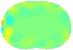
a)

b)

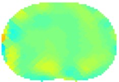
c)

d)

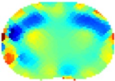
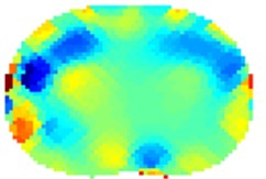
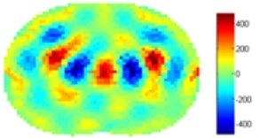
Fig. 5Results of volunteer breathing a) exhaling (frame 1), b) deep breath (frame 18

a)

b)

We have processed the measured data also using standard 2-norm approach. The results are on Fig. 5. The Gauss-Newton one step algorithm was used for reconstruction

For the case of Noser prior the right and left regions of lungs are more clearly visible but with very severe errors in the middle of each lung and in the middle of the trunk. We suspect that this can be attributed to algorithm artifacts. For the case of Laplace prior the results are very similar to the results of 1-norm presented in Fig. 4.

4. Conclusions

We have experimentally shown measurement of lungs on a volunteer. Since absolute imaging is very challenging, we have decided to use pseudo-differential imaging providing that reference image was taken when the volunteer exhaled as much air as possible. The results correspond well with expected phenomena. We were surprised to see the difference between the left and right lungs and we attribute this to heart and aorta. The standard deviation map can nicely visualize main activity inside the thorax cross-section. The results provided by EIT can be applied into clinical practice where a real-time monitoring of the patient at the bedside can help with individual adjustment of mechanical ventilation.