The application of fault diagnosis techniques and monitoring methods in building electrical systems – based on ELM algorithm

3.1. Fault simulation methods for building electrical systems and their feature quantity extraction

Fault diagnosis is actually the determination and identification of whether the system is operating abnormally. There are many different types of faults in building electrical systems and each fault is accompanied by abnormal data. Fault diagnostics instantly classifies and identifies the collected data and determines the indications and types of faults. However, any fault diagnosis method must be based on a basic modelling and data collection of the building electrical system and fault conditions. The study therefore starts with an analysis of the modelling of the building electrical system, fault simulation and extraction of characteristics.

When modelling building electrical systems, they need to be constructed according to their characteristics, as they are located in different environments, have different requirements and vary greatly in their functionality. In this study, the MATLAB/Simulink library is used to build a model of the electrical distribution system by selecting the appropriate model components and parameters [19]. Fig. 1 shows, for example, an extracted line topology of a lighting outlet in a hospital distribution system.

Fig. 1Building electrical system topology

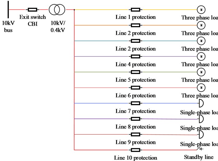
As can be seen from Fig. 1, the 10 kV busbar is the main network distribution line and CB1 is the distribution branch line switch. The main network current arrives at the distribution transformer via the branch line, which acts as a link between the low and high voltage sides and is used to step down the voltage from the high voltage side at 10 kV to the low voltage side at 0.4 kV. The building electrical system is modelled with a total of ten 0.4 kV outgoing lines, including six three-phase load fan coil lines and three single-phase load lighting-socket lines, as well as a standby line. To facilitate fault identification, a protection recording device was configured on each of these lines. The device is a three-phase voltage-current recorder, where the three-phase current and voltage values flowing through. Considering the economic constraints of the building electrical system, its sampling frequency is 20 kHZ. considering that the 10 kV system is generally a neutral point ungrounded system, set $Y$ as the way the three phase voltage source is grounded.

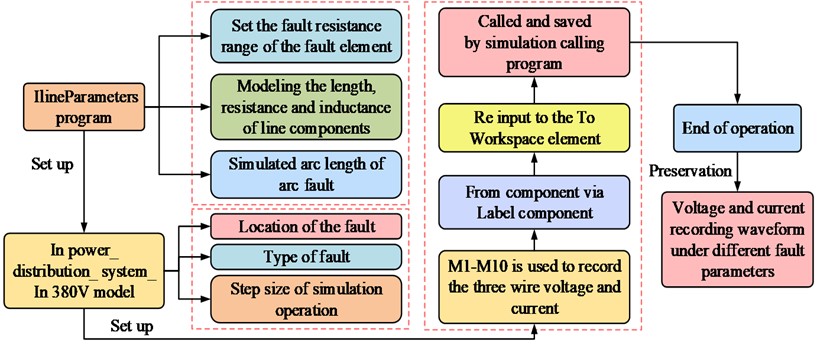
The parameter settings of the Powergui simulation master control element are related to the accuracy, effectiveness and time of the simulation. The study set the simulation method to discrete and the simulation time granularity to 5×10^-5 s. Single-phase fault elements were selected to implement different fault types. In the specific simulation process, the study uses the program loop call method to improve the efficiency with the flexibility of modelling and easy modification [20]. In this case, the fault parameters are set in the fault element as variables to be retrieved from the workspace. In the study, the resistance was set to FR for resistive faults and the arc length was set to LC for arc faults. All components were aggregated and connected according to the topology of the building electrical system topology diagram in it [21]. The steps required to model the building electrical system during the simulation run are shown in Fig. 2.

As shown in Fig. 2, the simulation process was mainly carried out to obtain the recorded voltage and current waveforms for different fault parameters. After summarizing the fault transient voltages and currents obtained from the simulation and their characteristics, the study proposes several characteristic quantities for fault identification in building electrical systems. Firstly, the three-phase voltage scaling capabilities reflect the information about the voltage change before and after the fault, and also the magnitude of the change. Therefore, the minimum value of the three-phase voltage is one of the most characteristic quantities for fault diagnosis in building electrical systems, which is calculated as in Eq. (1) [22]:

where, $U_{F_A}^{\mathrm{\text{'}}}$ represents the nominal value of the A-phase voltage after the fault, $u_{Fa}$ represents the magnitude of the A-phase voltage after the fault and $u_a$ is the magnitude of the A-phase voltage before the fault. The three phase currents are calculated as in Eq. (2) [23]:

where, $I_{F_A}^{\mathrm{\text{'}}}$ represents the post-fault A-phase voltage scale value, $i_{Fa}$ represents the post-fault A-phase voltage magnitude and represents the pre-fault A-phase voltage magnitude. The difference in the voltage expression of the arcing fault can then be highlighted by calculating the distortion of the three-phase voltage after the fault; the calculation is illustrated in Eq. (3) [24]:

where, $TH{D}_u$ represents the three-phase voltage distortion rate, $u_2$ to $u_n$ represent the 2nd to $n$ harmonic voltage rms values and $u_1$ represents the fundamental voltage rms values. The distortion rate of three-phase current after fault is then calculated as shown in Eq. (4) [25]:

where, $TH{D}_u$ represents the three-phase current distortion rate, $I_2$ to $I_n$ represent the 2nd to $n$ harmonic current rms, and $I_1$ represents the fundamental current rms. The above four indicators are used as the characteristic vectors for the types of orphaned airplane plunges in the building electrical system. After obtaining the waveforms of various obstacle recordings, the four indicators are then calculated for the three-phase voltage and current of each fault to obtain 12 fault diagnosis characteristic vectors.

Fig. 2Steps of building electrical system modeling in simulation operation

The fault characteristic quantity data obtained by studying the simulation and extraction of low-voltage building electrical systems include three-phase voltage after fault, three-phase current after fault, the distortion rate of three-phase voltage and three-phase current in 12 dimensions, and the types of simulated faults include 10 categories. Table 1 shows these types and numbers of building electrical fault diagnosis and monitoring simulation faults for this study.

3.2. Building electrical system fault diagnosis and monitoring construction based on ELM algorithm

After the basic simulation of the type and number of faults and the extraction of the characteristic quantities for the building electrical systems and fault states, the appropriate algorithm must be used to model them, and then the model must be used for fault identification and diagnosis. BP neural networks are widely used in current fault diagnosis due to their multi-hidden layer structure, which increases the computational power of diagnosis [26]. However, BP neural networks also have some obvious drawbacks, resulting in slow convergence of the computational results, or not easy convergence. The ELM method is based on the BP algorithm. The benefits of the ELM are based on its network structure and mathematical principles, which don't fix the number of neurons in the hidden layer but instead generate connection weights and thresholds at random between the input and hidden layers before continuously changing the number of neurons in the hidden layer to produce a theoretically distinct optimal solution [27]. First, the connection weights between the input and hidden layers are set according to Eq. (5):

where, $w_{ji}$ stands for connection weights between $i$ neuron of input layer and the $j$ neuron of the hidden layer. Similarly, the connection weights between implicit and output layer are shown in Eq. (6):

where, ${\beta }_{jk}$ is the connection weights between $i$ neuron of the input layer and $k$ neuron of the hidden layer. Set threshold of neuron transmission to the hidden layer be $b$, then its expression is shown in Eq. (7):

Set the data matrix of the training set with the number of samples $q$ be $X_{in}$, then its expression is shown in Eq. (8):

Similarly, the output matrix $Y_{out}$ is shown in Eq. (9):

When activation function is used for the neurons in hidden layer, let it be $g\left(x\right)$, then the network output $T$ is calculated as shown in Eq. (10):

where, $t$ is calculated as in Eq. (11):

In Eq. (12):

The above Eq. (12) can be simplified to Eq. (13):

where, $T^{\mathrm{\text{'}}}$ represents the transposed form of matrix $T$ and $H$ is output matrix of hidden layer of the ELM network, which is expressed as shown in Eq. (14)[28-29]:

Two important theorems have been proposed in the context of the underlying neural network structure. The first is that for a single-hidden-layer Feedforward Neural Network (SLFN) with $Q$ neurons, when faced with any $Q$ different samples, where $x_i=\left[{x_i}_1,{x_i}_2,\dots ,{x_i}_n\right]\in R^n$ and $t_i=\left[{t_i}_1,{t_i}_2,\dots ,{t_i}_m\right]\in R^m$ for an infinitely differentiable activation function $R:R\to$ R over a wide interval [30]. For randomly assigned weights $w_i\in R^m$ and thresholds $b_i\in R$, the output matrix $H$ is necessarily invertible for the hidden layer and has $‖H\beta -T^{\mathrm{\text{'}}}‖=0$. Second, when faced with any $Q$ number of different samples $\left(x_i,t_i\right)$, where $x_i={\left[x_{i1},x_{i2},\dots ,x_{i2}\right]}^T$ and $t_i=\left[x_{i1},x_{i2},\dots ,x_{i2}\right]\in R^m$. For any small error $\epsilon >0$ in a given environment, with an infinitely differentiable activation function $R:R\to$ R in any interval, there must exist an implicit layer SLFN containing a single neuron, with $‖H_{n*m}{\beta }_{M*m}-T^{\mathrm{\text{'}}}‖<\epsilon$ for randomly assigned weights $w_i\in R^m$ and thresholds $b_i\in R$ [31].

The ELM Extreme Learning Machine can be used in a stepwise manner when computing classification problems. The first step is to initialize the network with an input set of $X$ and an output set of $Y$. The output of the implicit layer is computed, and the connection weights and thresholds are computed through its input feature vector to obtain and the output of the implicit layer, which is expressed in Eq. (15):

For the output layer, the ELM neural network output value $T$ is calculated after accounting for the King City based on its structure by combining $H$, the connection weights $W_{jk}$ and the threshold $b$. The calculation is shown in Eq. (16):

Eq. (17) illustrates how ELN may approximate the training sample with 0 error performance for any weight and threshold when activation function $f\left(x\right)$ is an endlessly differentiable function if the number of neurons in the hidden layer is equal to the input in the actual problem:

It can be demonstrated that the error of the model derived from its training is incredibly small and is theoretically approximating the minimal value $\epsilon$, as shown in Eq. (18), when the number of neurons in the hidden layer benefits the number of inputs in the actual problem. At this point, the number of input sets appears to be too large:

The frontal network weights of the output and hidden layers are then updated. ELM keeps its network connection weights in a previously constant state during model training, but needs to update the weights of the output and hidden layers, as shown in Eq. (19):

where, $H^{+}$ is Moore Penrose generalized inverse matrix [32] of the implied layer output matrix $H$. The final step is to perform the iterative computation of this algorithm, as shown in Fig. 3.

Fig. 3Steps to establish ELM extreme learning machine

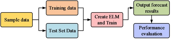
As seen in Fig. 3, the ELM is trained once a test set is produced. The ELM model is then tested by repeatedly iterating over the target accuracy values until the desired metric is obtained, resulting in the output of a performance evaluation of the ELM. If the set metric is not reached, the iterative computation continues. The study carried out model construction based on the above ELM algorithm principles, and structure of this model is shown in Fig. 4.

Fig. 4Fault identification and monitoring model of building electrical system based on ELM algorithm

As shown in Fig. 4, the study uses the ELM algorithm to monitor and identify faults in building electrical systems. Being a fault diagnosis model, the model has many inputs and a single output. At this point, the input to the model is a 12-dimensional feature vector. Experimental analysis of fault diagnosis technology and monitoring method for building electrical system based on ELM algorithm.

4.1. Transient analysis of building electrical system fault simulation

Since the number of hidden layer neurons of ELM extreme learning machine cannot be determined, the algorithm is needed to search automatically. The specific parameter Settings of ELM extreme learning machine, BP neural network and GA-BP neural network are shown in Table 2.

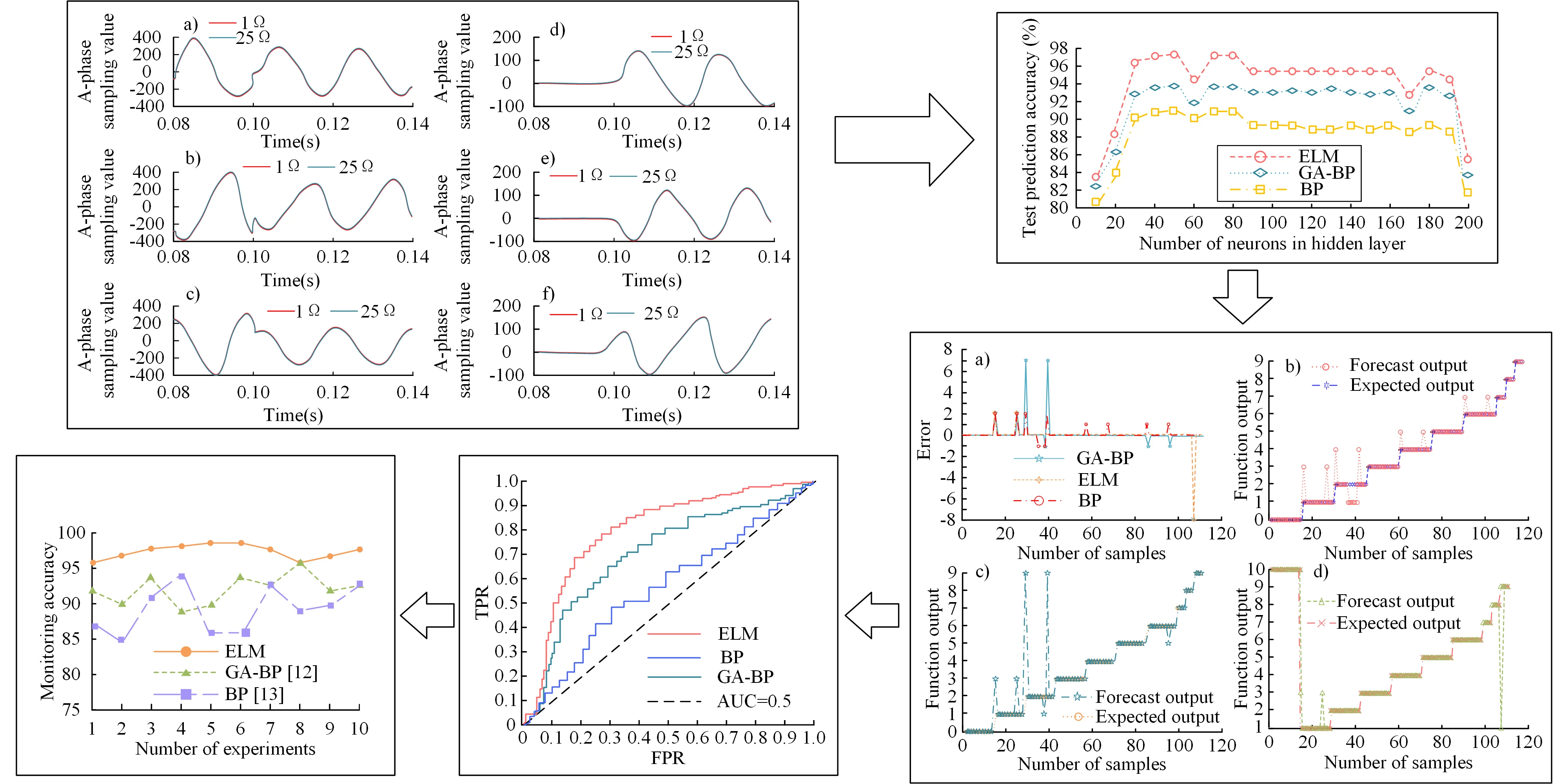
Fault simulations were performed on the modelled building electrical system, with the faults set to occur in the middle section of the line. For each type of fault in the model, several different sets of fault parameters were set to investigate the degree of change in system voltage and current and the trend under different fault parameters. This was done in an effort to simulate as closely as possible the faults that would occur in the field operation of the building electrical system. The wiring of the building electrical system was set up for an ABC three-phase short circuit fault. The fault resistance was varied from 1 Ω to 50 Ω, with a total of 50 sets of simulations. To highlight the contrast effect, only the transient voltage and current waveforms for the 1 Ω and 25 Ω simulations are drawn, as shown in Fig. 5. Note: Fig. 5(a) shows the A phase short-circuit fault simulation transient voltage. Fig. 5(b) shows the B phase short-circuit fault simulation transient voltage. Fig. 5(c) shows the C phase short-circuit fault simulation transient voltage. Fig. 5(d) shows the A phase short-circuit fault simulation transient current. Fig. 5(e) shows the B phase short-circuit fault simulation transient current. Fig. 5(f) shows the C phase short-circuit fault simulation transient current.

Fig. 5Waveform of transient voltage and current of three phase short circuit fault simulation

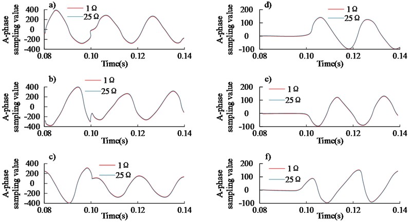
Fig. 5 shows that both the voltage and current of this system changed after a fault. The 1 Ω and 25 Ω simulated transient voltages showed the same trend, while the ABC three-phase short-circuit simulated voltage showed smaller fluctuations in the 0.07-0.1 s time range. Similarly, the 1 Ω and 25 Ω simulated transient currents showed almost no change in the 0.07-0.1 s time range. Similarly, the trends of the transient currents for the 1 Ω and 25 Ω simulations are consistent, but the ABC three-phase short circuit simulated currents show little variation in the 0-0.1 s time range and regular variation after 0.1 s. The results show that for a three-phase short circuit, the magnitude of this fault resistance has a limited effect on the three-phase voltage, but a greater effect on the three-phase current.

Due to the mechanistic nature of ELM learning, the number of neuron nodes is then selected after several matching trials. The effect of number of neurons in hidden layer on this ELM performance is shown in Fig. 6.

Fig. 6The influence of the number of hidden layer neurons on the performance of three algorithm models

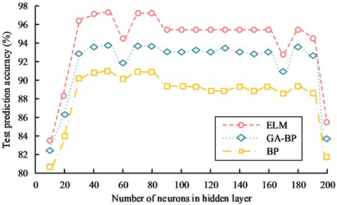
Fig. 6 illustrates how the ELM learning machine performs best when the number of hidden layer neuron nodes is set to 50, resulting in a test set prediction accuracy of approximately 97.86 %. As the number of neurons increased, the model's ability to generalise started to decrease. In the range of 85-160 neurons, the correct prediction rate was maintained at around 95.78 %. At 165 neurons in the hidden layer, it dropped to 92.34 %. After the number of neurons exceeded 180, the correct prediction rate of the model dropped sharply and overfitting occurred. Similarly, the prediction performance of the BP network model and the GA-BP network fault diagnosis model was affected by the number of neurons in the hidden layer, similar to that of the ELM-based model. When the number of hidden layers reached 50, the prediction accuracy of these two models was the highest, around 91.56 % and 93.69 % respectively. As the number of neurons in the hidden layer increases, the predictive ability of both models tends to decrease and eventually overfitting occurs. The experimental results showed that the ELM-based fault diagnosis model for building electrical systems was superior to other models in terms of prediction accuracy.

The 12 feature vectors were used as input to the fault diagnosis and monitoring model for this building electrical system and the studied ELM algorithm-based model was compared with the BP model and the Genetic Algorithm-Back Propagation (GA-BP) fault diagnosis model based on the Genetic Algorithm Optimization BP algorithm. The classification errors and classification outputs of the networked distribution network faults obtained from these three models are shown in Fig. 7. NOTE: Fig. 7(a) shows the classification error of three models. Fig. 7(b) shows the BP model classification output. Fig. 7(c) shows the GA-BP model classification output. Fig. 7(d) shows the ELM model classification output.

Fig. 7Fault classification results of distribution network based on ELM, BP and GA-BP algorithms

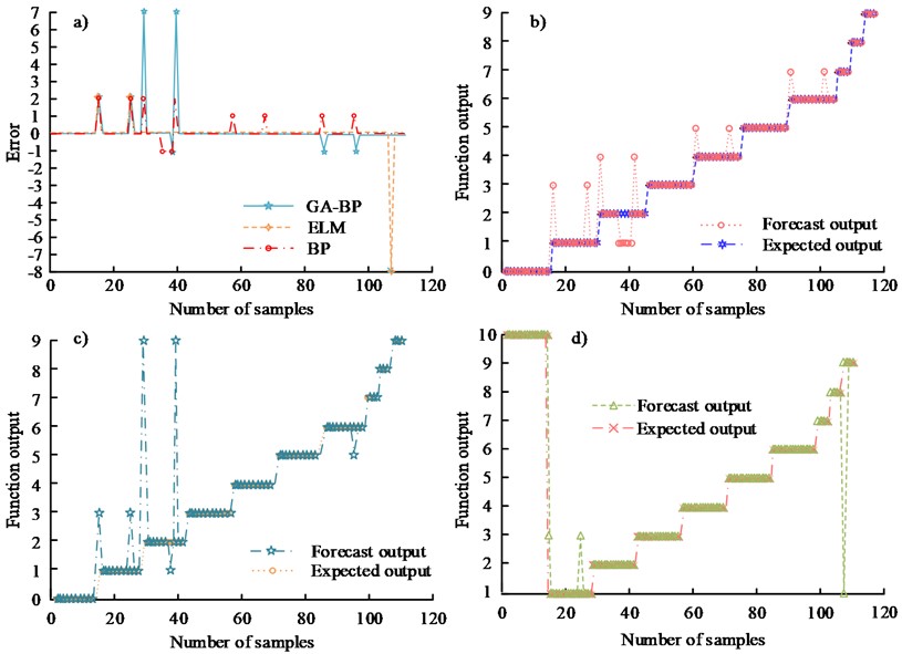
From Fig. 7(b), it can be seen this BP algorithm based model can accurately achieve the classification of 10 faults with a maximum error of 2. From Fig. 7(c), the GA-BP neural network based model can accurately achieve the classification of 10 faults with a maximum error of 7. From Fig. 7(d), the ELM algorithm based model can accurately achieve the classification of 10 faults with a maximum error of 2. From Fig. 7(a) and Fig. 7(b), it can be inferred that the model's classification accuracy for this sample is 89.09 %. Out of 110 samples, 12 of the anticipated results based on the BP neural network model had incorrect classifications. From Fig. 7(a) and Fig. 7(c), it can be seen that the predicted output based on the GA-BP algorithm model and the actual output error in 110 samples, there are 7 samples with Therefore, the classification accuracy of the model for this sample is 93.64 %. From Fig. 7(a) and Fig. 7(d), the predicted output of the ELM-based model is misclassified in only 2 out of 82 samples. Therefore, the classification accuracy of the model for this sample is 97.56 %. The results show that the ELM algorithm-based fault diagnosis technology and monitoring method for building electrical systems has a higher classification accuracy than both BP network and GA-BP model fault diagnosis models, showing better generalization ability and robustness.

To further validate the proposed method for fault detection in building electrical systems, it was compared with the BP and GA-BP models, respectively. The plot of the FPR-TPR binary is called the ROC curve, which makes it easier to determine the ability of a classifier to detect samples at a given threshold. The ROC curves of the three models are shown in Fig. 8.

Fig. 8ROC curves of three models

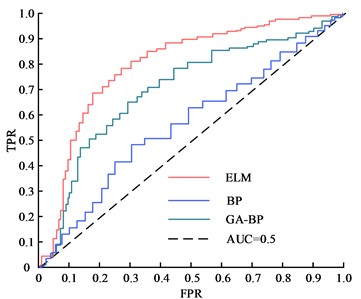
From Fig. 8, the AUC values of the research ELM algorithm-based model with BP model and GA-BP model are 0.92, 0.87 and 0.63, respectively. The results indicated that the research model was better than other two algorithm models for fault discrimination of building electrical systems.

4.2. Comparative analysis of performance of three fault diagnosis models for building electrical systems

Finally, to study the accuracy of the proposed methods for fault diagnosis of building electrical systems, they are compared with the BP and GA-BP models respectively. In order to avoid chance in calculation and to lessen the impact of random initial values on the results, the three methods are computed ten times to take the average value. Their performance comparison results are shown in Table 3. As the connection weights of its input and implied layers in ELM theory are random in nature.

Table 3 shows that the ELM algorithm has the lowest value for the root mean square error of fault classification, which is 0.3521. The GA-BP and BP algorithms have lower RMS errors of 0.2315 and 0.4402 lower respectively. The overall accuracy of ELM fault identification is much higher than the other two algorithms, being 3.63 % higher than the GA-BP algorithm and 8.18 % higher than the BP algorithm. In addition, in terms of running time, the ELM algorithm takes only 0.427 s, which is faster than the other two algorithms. In summary, the ELM algorithm has certain advantages over traditional algorithms in terms of recognition and running time.

As can be seen from Fig. 9, BP has a worse performance in terms of accuracy, comparing its results with those of ELM, the RMSE of BP is 0.4402 higher. The RMSE of the GA-BP model is 0.2315 higher than that of the ELM-based model. The ELM-based model has a 97.27 % correct rate in fault discrimination, which is better than other traditional or extended fault diagnosis monitoring models. In addition, the ELM model is faster in terms of model training time than the other models compared. As shown in Fig. 9, the monitoring accuracy of the research model is compared with the two more advanced fault diagnosis models in literature [12] and literature [13].

Fig. 9Monitoring accuracy comparison results of different models

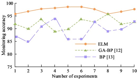
From Fig. 9, the ELM model data predicts small fluctuations, tends to be smooth and has a better monitoring accuracy of up to 98.6 %. Therefore, the proposed method can effectively and accurately diagnose and monitor the fault categories of building electrical systems and meet the real-time requirements. In summary, the ELM algorithm-based fault diagnosis and monitoring model for building electrical systems is optimal in terms of generalization performance, correct prediction rate and computation speed, and diagnosis and monitoring accuracy.